Fairness Principles

Slides — Chapter 2

Fei Huang, UNSW Sydney

Table of contents

• Step 1 — What is fair?
• Step 2 — Designing fair models
• Break — 10 min
• Steps 3 & 4 — brief overview
• Fairness for large language models

Today’s roadmap

2-hour session with five parts and five discussion breaks

Time	Part
0:00 – 0:45	Step 1: What is fair?
0:45 – 1:15	Step 2: Designing fair models
1:15 – 1:25	Break
1:25 – 1:40	Steps 3 & 4 (brief)
1:40 – 1:55	Fairness for large language models
1:55 – 2:00	Summary

Full detail lives in Lecture-Fairness-Principles.qmd. These slides are the in-class condensed version with discussion prompts built in.

Learning objectives

• Distinguish social, legal, and economic perspectives on fairness
• Compare quantitative fairness criteria and their assumptions
• Connect fairness criteria to model design and regulation
• Explain why no single criterion satisfies every stakeholder

Note

Insurance recurs as a worked example. The framework applies to any consequential automated decision.

Step 1 — What is fair?

The motivating problem

Case Study: COMPAS recidivism scoring

ProPublica’s Machine Bias investigation found Black defendants who did not reoffend were flagged “high risk” nearly twice as often as white defendants (Angwin et al. 2016).

The vendor countered that COMPAS was well-calibrated: same risk score, similar reoffense rate across race.

Has fairness been achieved? There’s no single answer. COMPAS is calibrated the same way for both groups, but its errors are not evenly distributed. Which one counts as “fair” depends on which of those two you prioritise.

This is not a coincidence of the COMPAS data. Whenever two groups reoffend, default, or claim at genuinely different rates, satisfying both sides at once becomes mathematically near-impossible, as this chapter makes precise later.

Both sides had a defensible claim, and that is exactly the problem. ProPublica’s critique was a separation-style argument, equal error rates across groups, and the vendor’s defence was a sufficiency-style argument, equal calibration across groups (Chouldechova 2017). A tool can satisfy one and violate the other, and choosing which to prioritise is the central question this chapter works through, not a modelling detail to resolve after the fact.

Three lenses on fairness

Lens	What it emphasises
Anti-discrimination	Legal obligation to avoid unjustified disparate outcomes
Competing ethical notions	Distributive justice, solidarity, pooling vs individualising
Consumer / user trust	Promises made in contracts, disclosures, conduct standards

These lenses don’t always agree. The point is making trade-offs visible before a model is built.

Feature principles

Using an input feature isn’t a purely statistical question:

• Control. Can the person influence it?
• Mutability. Fixed, or changes over time?
• Statistical discrimination. Does it predict the outcome?
• Causality. Does it cause the outcome?
• Past discrimination. Does using it reinforce history?
• Socially valuable behaviour. Does it discourage good actions?

Predictive power is necessary but not sufficient. A high-performing predictor can still be problematic on causality, history, or socially valuable behaviour, as with a credit score used in hiring or genetic testing used in insurance underwriting. Regulators have acted on this reasoning: 11 US states, most recently New York from April 2026, now restrict or ban employers from using credit checks in hiring, because credit history has no demonstrated causal link to job performance and reflects historical economic inequality (Martinez 2026).

Exercise: match example to principle

Match each example below to one of the six feature principles (Frees and Huang 2023):

1. Vehicle engine size predicts motor insurance claims frequency
2. A cancer diagnosis is known to cause elevated mortality risk
3. Ownership of a sports car, versus gender, race, ethnicity, or nationality
4. Basing insurance decisions on genetic test results
5. Age changes predictably over time, unlike place of birth
6. Discriminating on skin colour versus eye colour

No fragments here, work through it live with the class before advancing to the answers slide.

Answers: feature principles

1. Statistical discrimination — engine size has predictive value, which is necessary but not sufficient on its own

2. Causality — a known causal driver of the insured event

3. Control — sports car ownership is a choice, sensitive attributes are not

4. Socially valuable behaviour — discourages participating in genetic testing research

5. Mutability — changes over time versus staying fixed

6. Past discrimination — skin colour maps onto a protected, historically discriminated-against characteristic, eye colour does not

Direct and indirect discrimination

Direct (disparate treatment) means treated less favourably because a protected characteristic differs.

Indirect (disparate impact) means disproportionately affected because protected status is inferred through a neutral-seeming practice.

• Identifiable proxies, such as postcode↔︎race or résumé gaps↔︎caregiving status
• Unidentifiable proxies are opaque models reproducing disparities with no single surrogate

Case Study: algorithmic healthcare rationing

Removing the attribute isn’t enough

A hospital algorithm used healthcare cost as a proxy for need, to allocate care-management resources (Obermeyer et al. 2019).

Black patients historically had less access to care → lower costs for the same underlying need → the model systematically under-referred them, without ever using race as an input.

💬 Discuss (3 min)

Think of a variable, in a domain you know, that could be a proxy for a protected attribute.

Identifiable, or unidentifiable? Why does that distinction change how you’d fix it?

Indicative answers: proxy variables

A few examples across domains

Insurance: postcode as a proxy for race or socioeconomic status (identifiable, a single named column); claims-handling tone in free-text notes as a proxy for perceived credibility (harder to name, embedded in language).

Hiring: employment gaps as a proxy for caregiving status (identifiable); résumé-writing style learned from a demographically skewed training set (unidentifiable, no single feature to point to).

Lending: postcode or shopping patterns as a proxy for race (identifiable, the classic redlining pattern); an opaque credit score itself, if its inputs are undisclosed, can behave as an unidentifiable proxy even though it’s a single number.

Identifiable proxies can be found and removed (MCDP-style orthogonalisation, or dropping the variable). Unidentifiable proxies can’t be, since there’s no single column to act on, which is why testing outcomes directly (MDP, disparate-impact audits) matters more when the proxy is diffuse.

Fairness criteria: the taxonomy

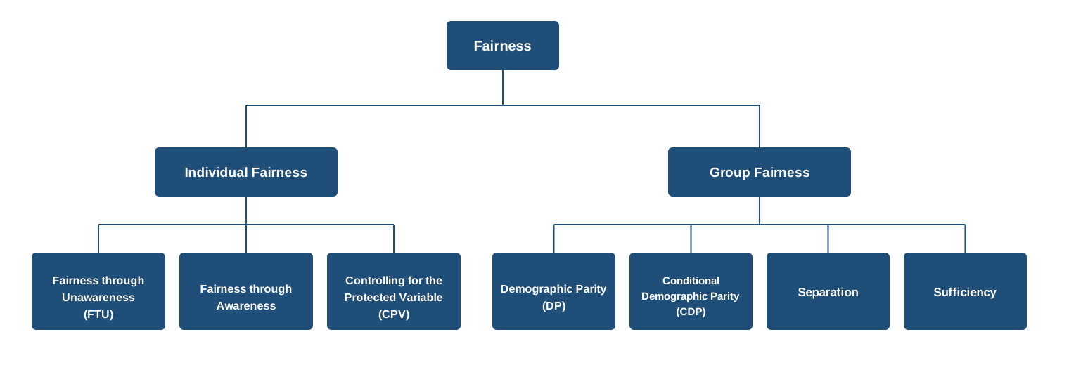
Fairness criteria: individual fairness

X_P = protected attribute, X_{NP} = other features, Y = actual outcome, \hat{Y} = prediction

Criterion	Formal condition	Intuition
FTU (fairness through unawareness)	\hat{Y} = f(X_{NP})	Remove the protected attribute
Fairness through awareness	D(\hat{Y}(x), \hat{Y}(y)) \le d(x, y)	Similar individuals get similar outcomes, via an explicit similarity metric d
CPV (controlling for the protected variable)	\hat{Y}_{CPV}(x) = E_{X_P}[f(x_{NP}, X_P)]	Average the model over X_P

Here x and y are two individuals (specific feature vectors), not the population-level X_P/X_{NP} used elsewhere in this table. \hat{Y}(x), \hat{Y}(y) are their predicted outcomes, d(x,y) measures how similar the two individuals are, and D measures how far apart their predictions are. Two similar individuals can’t get predictions further apart than their similarity allows.

FTU and fairness through awareness (Dwork et al. 2012) are general algorithmic-fairness concepts, applicable to any domain. CPV targets a different problem, proxy discrimination, where the protected attribute is excluded but its effect leaks through other variables. Developed for statistical profiling generally by Pope and Sydnor (2011) and adapted for insurance pricing as “discrimination-free pricing” by Lindholm et al. (2022).

Fairness criteria: group fairness

Criterion	Formal condition	Intuition
Demographic parity	\hat{Y} \perp X_P	Same outcome distribution, all groups
Conditional DP	\hat{Y} \perp X_P \mid X_{L}	Equal predictions within legitimate segments (segments defined by factors accepted as fair grounds for differentiation, covered later)
Separation	\hat{Y} \perp X_P \mid Y	Equal error rates across groups
Sufficiency	Y \perp X_P \mid \hat{Y}	Equal calibration across groups

\perp means statistically independent of (knowing one tells you nothing about the other). \mid means given, or within groups defined by.

Separation vs sufficiency

Separation asks whether, conditional on truth Y, errors are the same across groups.

Sufficiency asks whether, conditional on the prediction \hat{Y}, the truth is the same across groups.

Both are desirable, but generally can’t both hold when base rates (the actual outcome rate in each group) differ. (Except special cases, like perfect prediction.)

Naming the criteria

Event	Condition	Notion (\Pr\{\text{event} \mid \text{condition}\})
\hat{Y}=1	Y=1	TPR, recall
\hat{Y}=0	Y=1	FNR
\hat{Y}=1	Y=0	FPR
\hat{Y}=0	Y=0	TNR
Y=1	\hat{Y}=1	PPV, precision
Y=0	\hat{Y}=0	NPV

Same mechanism as the precision-recall trade-off, applied across groups instead of across thresholds. PPV is a function of TPR, FPR, and base rate, so matching TPR/FPR (recall) across groups with different base rates still leaves PPV (precision) unequal.

Separation is built from the first four rows (error rates conditioned on Y). Sufficiency is built from PPV (conditioned on Ŷ).

\Pr(\hat{Y} > t \mid Y = y, X_P = 0) = \Pr(\hat{Y} > t \mid Y = y, X_P = 1) for separation. \Pr(Y = y \mid \hat{Y} = s, X_P = 0) = \Pr(Y = y \mid \hat{Y} = s, X_P = 1) for sufficiency. This is the COMPAS tension from Chapter 1, calibrated (sufficiency) but unequal error rates (violates separation).

💬 Discuss (3 min)

In practice, you usually can’t satisfy both separation and sufficiency at once, and have to prioritise one.

What would you look at to decide which one to prioritise for a given decision?

Indicative answer: separation vs sufficiency

What the literature suggests

The relative cost of the two error types. Equalised-odds-style separation was originally motivated by asymmetric error costs (Hardt et al. 2016). If a false positive (e.g. wrongly denying parole) is a much worse harm than a false negative, prioritise equalising that error rate across groups rather than full calibration.

Whether a human interprets the score downstream, or a fixed threshold gates the decision automatically. A score a human consults (e.g. a risk score shown to a judge) needs to mean the same thing for every group, which is what calibration guarantees, so sufficiency matters more. A score that triggers an automatic cutoff is better served by equal error rates at that cutoff, which is what separation guarantees.

What the original COMPAS debate actually turned on. ProPublica’s separation-style critique focused specifically on FPR, the rate at which defendants who did not reoffend were nonetheless flagged high-risk, a punitive error. Northpointe’s sufficiency-style defence focused on calibration, arguing the score meant the same thing for every defendant. Neither side was wrong about the criterion they picked; they disagreed about which error mattered more (Kleinberg et al. 2017; Chouldechova 2017).

Incompatibility of criteria

Individual and group fairness together are often impossible to achieve simultaneously.

This is exactly the COMPAS tension from the start of this chapter. ProPublica’s critique was separation-style, the vendor’s defence was sufficiency-style. Both were valid, and neither could hold at once given the different reoffense base rates across race.

This is a special case of a more general result (Kleinberg et al. 2017): except in narrow special cases, no classifier can simultaneously satisfy calibration and balanced error rates across groups when the groups have different base rates.

Why base rates force the trade-off

\text{PPV}_g = \frac{p_g(1 - \text{FNR}_g)}{p_g(1-\text{FNR}_g) + (1-p_g)\,\text{FPR}_g}

• If separation holds, FPR and FNR are the same in both groups, so PPV depends only on the base rate p_g
• Sufficiency needs equal PPV across groups, which then forces p_0 = p_1
• COMPAS: two-year reoffense rate was 51% for Black defendants, 39% for White defendants (Chouldechova 2017), so p_0 \neq p_1

Equally reliable “high risk” flags in both groups, but different reoffense rates, mean different false positive rates. That’s algebra, not evidence of biased predictions.

Except at the two degenerate extremes, a perfect classifier where FPR = FNR = 0, or one that ignores the data entirely, separation and sufficiency cannot both hold once base rates differ. Worth walking through slowly: PPV is what sufficiency/calibration asks to be equal. Holding FPR and FNR fixed (that’s separation) turns PPV into a function of the base rate alone, so equal PPV across groups collapses to requiring equal base rates, which COMPAS does not have.

Confusion matrices

100 people per group, same FNR (10%) and FPR (20%) in both, so separation holds by construction.

Group A

	Predicted \hat{Y}=1	Predicted \hat{Y}=0
Actual Y=1	TP = 27	FN = 3
Actual Y=0	FP = 14	TN = 56

Group B

	Predicted \hat{Y}=1	Predicted \hat{Y}=0
Actual Y=1	TP = 54	FN = 6
Actual Y=0	FP = 8	TN = 32

Worked example

\text{Flag rate}_g = \frac{TP+FP}{TP+FP+FN+TN} \quad \text{TPR}_g = \frac{TP}{TP+FN} \quad \text{FPR}_g = \frac{FP}{FP+TN} \quad \text{PPV}_g = \frac{TP}{TP+FP}

	Group A (p_0 = 30%)	Group B (p_1 = 60%)
Reoffend	30	60
Do not reoffend	70	40
Correctly flagged	27	54
Wrongly flagged	14	8
Total flagged high-risk	41	62
Flag rate (demographic parity)	41%	62%
\text{TPR}_g,\ \text{FPR}_g (separation)	90%, 20%	90%, 20%
PPV_g (sufficiency)	27/41 ≈ 66%	54/62 ≈ 87%

Same error rates, but flag rate differs (41% vs 62%) and PPV jumps from 66% to 87%, purely from the base-rate gap. Matching flag rate or PPV instead would each require different FPR/FNR in each group, violating separation.

Matching criterion to regime:

• Prohibition on X_P → FTU.
• Proxy discrimination (protected variable not used, but its effect leaks through correlated variables) → CPV, e.g. Colorado’s SB21-169 and New York’s DFS Circular Letter No. 7 (Colorado General Assembly 2021; New York State Department of Financial Services 2024).
• Prohibition on proxies too → MU* (MU extended to also drop named proxy variables). Colorado’s SB21-169 testing regime is also the clearest regulatory example of conditional demographic parity in practice (Colorado General Assembly 2021).
• EU unisex insurance pricing → same price for the same rating profile, an individual-level condition. FTU and CPV both satisfy it directly.

CPV is not a blanket ban on the protected variable, it targets proxy discrimination: cases where the protected variable itself is excluded but other variables still carry its effect. Colorado requires insurers to test predictive models for unfair discrimination arising from this kind of proxy effect; New York imposes similar expectations for AI systems and external data used in underwriting and pricing.

MU* extends MU by also removing rating variables explicitly named as proxies for X_P under a specific regulation, rather than X_P alone. Plain MU leaves those variables untouched. MU* still leaves unnamed or statistically inferred proxies untouched, which is what MCDP and MDP are designed to catch.

Two logics of resource allocation

Position	Emphasis	Logic
Social good	Solidarity, access, universal service	Subsidising solidarity
Economic commodity	Efficiency, adverse selection	Chance solidarity

Actuarial fairness and the EU gender ban

Actuarial fairness means charging each insured person only for their own risk. In the EU’s 2012 ban on gender-based motor pricing, the ECJ held that equal treatment took precedence over gender being a statistically valid predictor (European Court of Justice 2011). The ban didn’t remove the underlying risk difference — it redistributed who pays for it.

Adverse selection means higher-risk people are more likely to buy insurance, since they know their own risk better than the insurer does. Subsidising solidarity pools costs across everyone regardless of individual risk. Chance solidarity pools the shared uncertainty of who will have a claim, while pricing still tracks individual risk.

Consumer / user trust

• Information asymmetry, since the user discloses while the org holds far more data (formalised in insurance as “utmost good faith”: a duty for both sides to disclose relevant facts honestly)
• Compliant ≠ fair-feeling, if it diverges from disclosed promises
• Outcome-irrelevant differentiation means pricing on shop-around likelihood, not actual risk, and it’s contested when it correlates with a protected attribute

Compliance with anti-discrimination rules is necessary but not sufficient for this lens.

💬 Discuss (4 min)

Separation and sufficiency can’t both hold when base rates differ.

If you had to pick one, for a domain you care about — which, and what are you trading away?

Indicative answer: applying the trade-off

Two examples, using the framework from Step 1

Criminal-justice risk scoring (like COMPAS): a false positive (wrongly flagged high-risk) is a punitive harm affecting someone’s liberty. This pushes toward separation, specifically equalising FPR, even at the cost of calibration.

Medical risk scoring (e.g. a score a clinician uses to prioritise screening): the score is interpreted by a human downstream, and a “70% risk” that means different things by group directly undermines clinical trust. This pushes toward sufficiency: calibration matters more than matching error rates exactly.

Whichever you pick, name what you’re giving up. That’s the actual skill this chapter is teaching: not “solving” the trade-off, but making the choice, and its cost, explicit and defensible.

Step 2 — Designing fair models

How is fairness enforced?

Stage	What happens	Models
Pre-processing	Adjust inputs before training	MDP, MCDP
In-processing	Build fairness into the objective	Constrained optimisation
Post-processing	Adjust outputs after training	MC

The right stage depends on the criterion chosen in Step 1, not what’s easiest to implement. MDP/MCDP/MC are this course’s named examples per stage. The same criterion could in principle be reached by a different route (Barocas et al. 2023, ch. 3).

The five model designs

Model	Criterion	Approach
M0	Baseline	Uses X_P and X_{NP}
MU	FTU	Protected attribute removed
MDP	Demographic parity	Debias all X_{NP}
MCDP	Conditional DP	Debias only non-legitimate predictors
MC	CPV	Fit M0, then average over X_P at scoring

Step 1’s criteria came from a classification example (COMPAS). Insurance pricing is usually regression — Xin and Huang (2024) formalise these five designs for continuous \hat{Y} (claim frequency, severity, pure premium). DP extends directly (equal average \hat{Y} across groups); separation/sufficiency’s TPR/FPR/PPV form needs a continuous-outcome analogue instead.

No confusion matrix once \hat{Y} is continuous — TPR/FPR/PPV don’t apply directly. The underlying idea (equal error rates for separation, equal calibration for sufficiency) still generalises, but the exact formula has to be adapted. The five designs (M0-MC) don’t care which criterion, or which extension of it, you pick — same toolkit either way.

Formal definitions

Notation from Xin and Huang (2024): X_{NP}^* is debiased X_{NP}, X_{NP_{legit}} / X_{NP_{not}} split X_{NP} for MCDP.

\hat{Y}_{M0} = f_{M0}(X_{NP}, X_P) \hat{Y}_{MU} = f_{MU}(X_{NP}) \hat{Y}_{MDP} = f_{MDP}(X_{NP}^*) \hat{Y}_{MCDP} = f_{MCDP}(X_{NP_{not}}^*,\, X_{NP_{legit}}) \hat{Y}_{MC} = \frac{1}{N}\sum_{j=1}^N \hat{f}_{M0}(X_{NP},\, X_P = x_{P_j})

X_{NP}^* construction: orthogonal-predictors method, regress X_{NP} on X_P, take residual, X_{NP}^* = X_{NP} - \hat{X}_{NP} — first proposed for insurance pricing by Frees and Huang (2023). M0/MDP/MCDP need X_P at both training and prediction; MC needs it only at training, since prediction uses the population-average x_{P_j} rather than the individual’s own value.

MDP: \tilde{X}_j = X_j - E[X_j \mid X_P], train on residuals. This ensures \hat{Y} \perp X_P by construction, but only removes the mean dependence on X_P. Optimal transport (Lindholm et al. 2024b) remaps the full distribution instead, more thorough but more computationally involved (Kamiran and Calders 2012, Kamiran and Calders (2012)). MCDP: same debiasing, only on non-legitimate predictors X_{NL}, \tilde{X}_{NL} = X_{NL} - E[X_{NL} \mid X_P, X_L]. This allows variation through legitimate factors. MC: fits M0 in full, then averages out X_P at scoring time, \hat{Y}_{MC}(x) = \frac{1}{N}\sum_j \hat{f}_{M0}(x_{NP}, X_P=x_{P_j}). This removes direct effects while preserving accuracy on other features.

Pre-processing (MDP, MCDP) guarantees the criterion regardless of downstream training (data-processing inequality), but only for the criterion it was built for. In-processing (constrained optimisation, e.g. Lindholm et al. (2024a)’s multi-task network) can reach the best accuracy for a given fairness level since the constraint is optimised for directly, but needs access to the training pipeline. Post-processing (MC) works on any trained black-box model with no retraining, and can be provably optimal if the underlying score is already Bayes-optimal, but it explicitly uses group membership at the point of decision.

Legitimate vs non-legitimate variables

Legitimate means grounds a regulator/institution accepts for differentiated treatment.

• Insurance: claims history, vehicle type ✓ · fine-grained geography ✗ (some markets)
• Lending: income, repayment history ✓ · postcode alone ✗
• Hiring: role-relevant skills ✓ · protected-attribute proxies ✗

MCDP is built for this. Differences allowed only through legitimate variables.

How regulation maps to model design

No restriction → M0 · Prohibit X_P → MU · Prohibit proxies too → MU* · Equal average outcomes → MDP · Full pooling → community rating (same price for everyone in a group regardless of individual risk)

Note

Not every regulation maps to one criterion cleanly, common under principles-based regimes: China’s NFRA guidance (National Financial Regulatory Administration 2026a, 2026b; Sina Finance 2026), Australia’s AHRC (Australian Human Rights Commission and Actuaries Institute 2022), and Singapore’s MAS FEAT/Veritas (Monetary Authority of Singapore 2018, 2019) all avoid prescribing a single fairness criterion. The institution has to choose, using Step 1’s judgement.

The fairness–accuracy trade-off

French motor insurance evidence (Xin and Huang 2024):

• MCDP and MC show loss ratios (the share of premium income paid out in claims) close to unconstrained M0
• Accuracy loss: modest
• Disparity reduction: substantial
• XGBoost retained most of its edge while meeting fairness criteria

The cost of fairness is smaller than often assumed, but not zero. Strict demographic parity trades off against something like adverse selection. Quantifiable, but still a business decision.

The same modest-accuracy-loss pattern recurs beyond insurance. Rodolfa et al. (2021) find it across education, mental health, criminal justice, and housing safety. Hardt et al. (2016) find a similar pattern in credit scoring. Mehrabi et al. (2021) surveys the broader evidence.

The trade-off, visualised

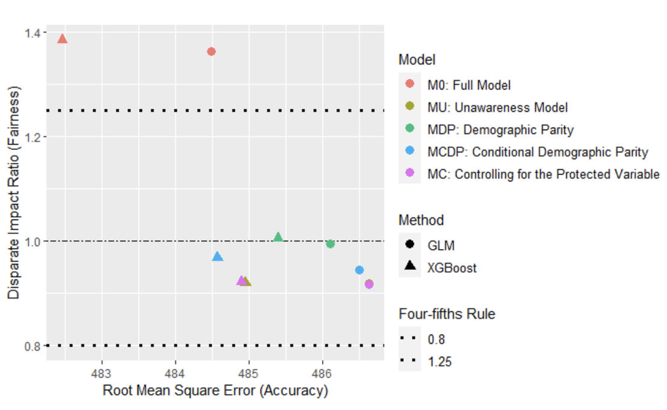
Root mean square error (x, lower is more accurate) vs. disparate impact ratio (y, 1 is perfect parity), five model designs, GLM and XGBoost, French motor insurance data (Xin and Huang 2024). Dotted lines mark the four-fifths rule’s 0.8–1.25 band.

M0 (uses the protected attribute) is the most accurate point on the plot but sits furthest outside the four-fifths band. MDP and MCDP pull the ratio back toward 1 for a small RMSE cost. MCDP and MC push slightly below 1, still at small accuracy cost relative to M0. MU happens to land inside the band on this dataset too, which is a property of this dataset’s proxy structure, not a general guarantee. It’s why FTU is necessary but not sufficient.

💬 Discuss (4 min)

The insurance case study found only a modest accuracy cost for fairness.

Do you think that generalises, or is it domain-specific? What would make the trade-off worse?

Indicative answer: does the modest trade-off generalise?

Evidence points both ways

Supporting generalisation: Rodolfa et al. (2021) find the same modest-cost pattern across education, mental health, criminal justice, and housing safety; Hardt et al. (2016) find it in credit scoring too. Several independent domains, same qualitative result.

Against blanket generalisation: the cost depends on how much of a model’s predictive power is actually carried by the protected attribute or its correlates. A large base-rate gap between groups (like COMPAS’s) means removing or orthogonalising that signal costs more. A weak correlation means fairness is closer to free.

What would make it worse: smaller training data (less signal to substitute for the removed correlation), a narrower feature set, or a genuinely strong relationship between the protected attribute and the outcome that the model can’t recover elsewhere.

Break — 10 min

Steps 3 & 4 — brief overview

Step 3: downstream impact

A model meeting its criterion can still produce an unfair outcome once its predictions hit a real process.

A downstream step, re-ranking, a discretionary override, a separate margin or eligibility adjustment, can undo fairness achieved at the model stage if it correlates with a protected group.

Same structure in hiring, pricing, and lending, wherever a fair model’s output is adjusted afterward by a separate, unconstrained layer. fair.feihuang.org Step 3 covers the welfare-analysis methods that quantify this.

Step 4: auditing the system

Audit asks whether we can demonstrate compliance. Test asks whether we can find a problem.

A credible audit:

• Pre-commits its test, tolerance, control variables before looking at the data
• Uses equivalence testing (TOST), not a conventional significance test
• Puts the burden of proof on the organisation, not the regulator

TOST (two one-sided tests) checks whether a difference is small enough to fall within an acceptable range, rather than testing whether it differs from zero the way a standard significance test does.

A separate, older tradition tests blindness directly. It sends matched pairs through the real decision-making system that differ only in the attribute of interest (e.g. an otherwise-identical résumé with a Black-sounding versus White-sounding name), and compares outcomes (Barocas et al. 2023, ch. 7). This is the design behind classic audit studies like Bertrand and Mullainathan’s résumé study, and it’s also the design behind the LLM case study coming up. Huang et al. (2026) hold everything but the claimant’s stated gender fixed and compare the model’s output.

Fairness for large language models

Where the bias comes from

No fixed input schema. No column called “Gender,” prediction is open-ended text.

• Shaped by the training corpus, which reproduces whatever stereotypes are in the text
• Further shaped by alignment fine-tuning (e.g. RLHF, reinforcement learning from human feedback), which encodes the labellers’ preferences
• No single attribute to remove. Bias surfaces in word choice, tone, assumed perspective

Why measurement is harder

Group-fairness criteria compare a well-defined \hat{Y} across groups.

Open-ended generation has no single \hat{Y}. Evaluation needs templated probes (swap a name/pronoun, compare sentiment/toxicity).

Dozens of proposed metrics, little consensus (Gallegos et al. 2024). This is considerably less mature than the tabular setting this course focuses on.

💬 Discuss (3 min)

A conventional bias audit compares outcomes for Male vs. Female claimants only, since that’s how gender has traditionally been recorded.

Real intake forms increasingly offer Non-binary and “prefer not to say” options too. If an LLM passed a Male/Female audit with no disparity, would you trust it to be unbiased for the categories the audit never tested? What could go wrong that a binary audit would miss entirely?

Case Study: gender bias in LLM insurance claims — the design

Huang et al. (2026)’s counterfactual audit:

• 1,388 real vehicle insurance claims (accident image, vehicle metadata, optionally an AI-generated narrative)
• 4 gender conditions: Male, Female, Non-binary, Not Specified, not just the conventional Male/Female binary
• 2 × 2 further conditions: claimant’s name present/absent, narrative present/absent
• 6 LLMs: GPT-5, GPT-4o, Gemini 2.5 Pro, Gemini 3 Flash, Claude 4 Sonnet, Claude 4.5 Sonnet
• 3 outcomes per claim: predicted claim amount, eligibility, damage severity
• 4 \times 2 \times 2 \times 1{,}388 \times 6 \times 3 \rightarrow 133,248 model evaluations

Everything about the claim is held fixed except the gender field and the two prompt conditions, a counterfactual design, the same logic as the résumé-audit technique covered earlier in this chapter.

Case Study: gender bias in LLM insurance claims — results

Under the conventional Male/Female, full-information audit: none of the six models shows a significant disparity.

Once Non-binary and Not Specified are included, three models (GPT-5, GPT-4o, Gemini 2.5 Pro) show significant disparities. GPT-4o is the most biased: $128–$288 difference in predicted claim amount, favouring Not Specified claimants when the name is present, but the disparity flips to favour Non-binary over Male claimants once the name is removed.

Three models (Gemini 3 Flash, Claude 4 Sonnet, Claude 4.5 Sonnet) show no significant disparity under any of the 16 conditions tested.

A binary-only audit would have certified all six models as fair.

Exercise: how would you fix this?

GPT-4o shows the bias; three other models (Gemini 3 Flash, Claude 4 Sonnet, Claude 4.5 Sonnet) don’t.

Before the next slide: as the insurer’s AI governance lead, what would you actually change? List at least two concrete options.

Indicative answer: fixing the LLM insurance-claims bias

Options grounded in the paper and this chapter

Change the prompt, not just the model. GPT-4o’s bias pattern flips depending on whether the claimant’s name is present. Stripping the name (and other demographic-adjacent free text) from the prompt before the claim reaches the model is the LLM analogue of FTU, removing an input the model doesn’t need to do its job.

Switch models, if procurement allows it. Three of the six models tested show no significant disparity under any condition. Model choice is itself a fairness lever, not just a technical one, provided switching doesn’t trade away needed capability.

Audit is not a one-off gate. GPT-5 fixed most of GPT-4o’s disparities, but that isn’t guaranteed for every update. Every model version change should trigger a new, multiplicity-aware audit (multiple gender categories, multiple prompt configurations), not a one-time sign-off at procurement.

Notice what’s missing: there’s no MCDP-style pre-processing step. The LLM’s input isn’t a fixed feature vector X_{NP} you can orthogonalise, so the five-model toolkit from Step 2 doesn’t transfer directly to open-ended generation.

💬 Discuss (3 min)

Real-estate platforms are starting to use GenAI to suggest listing prices.

Historically, human-set housing prices have been higher in white-dominant neighbourhoods than in comparable minority-dominant ones. If an LLM is trained on this same historical data, would you expect its prices to reproduce, widen, or narrow that gap? Why?

Case Study: GenAI and housing price discrimination — the design

Tanlamai et al. (2026)’s comparison:

• 284,749 real U.S. property listings (Aug–Sep 2023), across five property types
• Each listing’s human-set asking price is the baseline
• GPT-4o is prompted to act as a real-estate agent and generate its own price for the same listing, from the same characteristics (location, size, beds/baths, school rating, climate-risk scores)
• Neighbourhoods classified white-dominant (>50% white residents) or minority-dominant, from Census Bureau data
• A fixed-effects regression on \log(\text{Price}) compares human vs. GenAI prices, controlling for property characteristics, house type, and city
• Robustness checked across 4 LLMs: GPT-4o, GPT-3.5, Gemini 1.5 Flash, Claude 3.5 Sonnet

Case Study: GenAI and housing price discrimination — results

Human-set prices: houses in minority-dominant neighbourhoods are priced 22.9% lower than comparable houses in white-dominant neighbourhoods.

GPT-4o prices: the same gap shrinks to 14.2%, an 8.7 percentage-point reduction, not an amplification.

GenAI prices are lower than human prices overall (13.5% lower on average), but the reduction is larger for minority-dominant neighbourhoods, which is what narrows the gap.

The opposite direction from the insurance case study. Mechanism checks suggest it isn’t just “regression to the mean”: it’s driven by what the training data (much of it public web content) encodes about pricing generally, not a simple averaging effect.

Exercise: how would you fix this?

GPT-4o narrows the racial pricing gap (22.9% → 14.2%), but doesn’t eliminate it.

Before the next slide: would you deploy GPT-4o’s prices as-is, or add a correction step? What would that correction look like, using this chapter’s own toolkit?

Indicative answer: fixing the residual housing-price gap

Options grounded in this chapter

Treat the residual 14.2% gap as an unfinished Step 2 problem, not a solved one. GPT-4o’s price is a fitted output over X_{NP} (location, size, school rating, and so on), so it can be treated like any other predicted price for this chapter’s toolkit.

MCDP-style correction: identify which of GPT-4o’s inputs are legitimate risk factors (e.g. flood risk, school rating) versus non-legitimate proxies (e.g. a postcode standing in for neighbourhood racial composition), and orthogonalise only the latter against race before the price is finalised.

MC-style correction: average GPT-4o’s price over the neighbourhood’s racial composition at scoring time, the same post-processing idea used in the insurance-pricing worked example earlier in this chapter.

Neither is free. Both require the platform to first classify legitimate vs. non-legitimate inputs (a judgement call) or to have race/neighbourhood-composition data available at scoring time, exactly the same practical costs already discussed for MCDP and MC.

💬 Discuss (3 min)

If you were auditing an LLM drafting claim-denial letters —

what would “fair” even mean here, with no single \hat{Y} to compare?

Indicative answer: fairness for open-ended text

No single Ŷ, but not undefined either

Templated probes, not direct criteria. Hold the claim details fixed, swap only the claimant’s name or stated demographic, and compare the generated text across the swap: tone (via sentiment analysis), specificity of the stated denial reason, or presence of an appeals-process explanation.

Decompose “fair” into measurable proxies. Even without a single outcome number, ask: is the rate of denial letters (a binary extractable from the text) equal across groups, a demographic-parity-style question? Is the letter’s reading level or actionability, a proxy for how easy it is to contest the decision, equal across groups?

This is exactly Gallegos et al. (2024)’s point: dozens of proposed metrics exist because no single one dominates. The audit design has to be built for the specific harm, not borrowed wholesale from the tabular setting.

Summary: the four-step framework

Step	Question	Depth here
1. Define fairness	Which criterion applies?	Full
2. Design a fair model	Which design enforces it?	Full
3. Assess impact	Who gains/loses in practice?	Brief
4. Audit the system	Can we demonstrate compliance?	Brief

💬 Discuss (5 min) — wrap-up

Of the four steps — define, design, assess impact, audit —

which do you think organisations skip most often in practice, and why?

Indicative answer: which step gets skipped

Most commonly nominated: Step 4 (audit)

Steps 1 and 2 are where the interesting technical work happens, and where a data science team’s incentives naturally point, so they tend to get done. Step 3 (impact assessment) is at least partially forced by growing algorithmic-impact-assessment regulation. Step 4 (ongoing audit) is the one most often skipped, because it has no natural endpoint (a model “passes” once at deployment, but nothing forces a recheck later), and because, as the LLM case study earlier in this chapter showed, a model that passes today’s audit can fail tomorrow’s after a routine version update.

Recommended reading

• Xin and Huang (2024) — criteria, model designs, trade-off on insurance data
• Barocas et al. (2023) — Fairness and Machine Learning (free, fairmlbook.org)
• Gallegos et al. (2024); Huang et al. (2026); Tanlamai et al. (2026) — fairness specifically in LLMs

Full list, including fair.feihuang.org’s interactive tools, in the lecture notes.

Next class

Chapter 3 — Fairness Practice

Bring a laptop with R installed. We’ll fit these five model designs on real data.

Angwin, Julia, Jeff Larson, Surya Mattu, and Lauren Kirchner. 2016. “Machine Bias.” ProPublica. https://www.propublica.org/article/machine-bias-risk-assessments-in-criminal-sentencing.

Australian Human Rights Commission and Actuaries Institute. 2022. Guidance Resource: Artificial Intelligence and Discrimination in Insurance Pricing and Underwriting. https://humanrights.gov.au/resource-hub/by-resource-type/publications/technology-and-human-rights/guides/guidance-resource-ai-and-discrimination-insurance.

Barocas, Solon, Moritz Hardt, and Arvind Narayanan. 2023. Fairness and Machine Learning: Limitations and Opportunities. MIT Press. https://fairmlbook.org.

Chouldechova, Alexandra. 2017. “Fair Prediction with Disparate Impact: A Study of Bias in Recidivism Prediction Instruments.” Big Data 5 (2): 153–63. https://doi.org/10.1089/big.2016.0047.

Colorado General Assembly. 2021. Senate Bill 21-169: Protecting Consumers from Unfair Discrimination in Insurance Practices. Colorado Division of Insurance. https://doi.colorado.gov/for-consumers/sb21-169-protecting-consumers-from-unfair-discrimination-in-insurance-practices.

Dwork, Cynthia, Moritz Hardt, Toniann Pitassi, Omer Reingold, and Rich Zemel. 2012. “Fairness Through Awareness.” Proceedings of the 3rd Innovations in Theoretical Computer Science Conference, 214–26.

European Court of Justice. 2011. Judgment of the Court (Grand Chamber) of 1 March 2011, Association Belge Des Consommateurs Test-Achats ASBL and Others v Conseil Des Ministres. Case C-236/09. https://eur-lex.europa.eu/legal-content/EN/ALL/?uri=CELEX%3A62009CJ0236.

Frees, Edward W, and Fei Huang. 2023. “The Discriminating (Pricing) Actuary.” North American Actuarial Journal 27 (1): 2–24.

Gallegos, Isabel O, Ryan A Rossi, Joe Barrow, et al. 2024. “Bias and Fairness in Large Language Models: A Survey.” Computational Linguistics 50 (3): 1097–179.

Hardt, Moritz, Eric Price, and Nati Srebro. 2016. “Equality of Opportunity in Supervised Learning.” Advances in Neural Information Processing Systems 29.

Huang, Fei, Md Mushahidul Islam Shamim, Warut Khern-Am-Nuai, and Maxime C. Cohen. 2026. “Beyond the Binary: Gender Bias in LLM-Evaluated Insurance Claims.” https://ssrn.com/abstract=7127259.

Kamiran, Faisal, and Toon Calders. 2012. “Data Preprocessing Techniques for Classification Without Discrimination.” Knowledge and Information Systems 33 (1): 1–33.

Kleinberg, Jon, Sendhil Mullainathan, and Manish Raghavan. 2017. “Inherent Trade-Offs in the Fair Determination of Risk Scores.” Proceedings of the 8th Innovations in Theoretical Computer Science Conference.

Lindholm, Mathias, Ronald Richman, Andreas Tsanakas, and Mario V Wüthrich. 2022. “Discrimination-Free Insurance Pricing.” ASTIN Bulletin: The Journal of the IAA 52 (1): 55–89.

Lindholm, Mathias, Ronald Richman, Andreas Tsanakas, and Mario V Wüthrich. 2024a. “A Multi-Task Network Approach for Calculating Discrimination-Free Insurance Prices.” European Actuarial Journal 14: 329–69.

Lindholm, Mathias, Ronald Richman, Andreas Tsanakas, and Mario V Wüthrich. 2024b. “What Is Fair? Proxy Discrimination Vs. Demographic Disparities in Insurance Pricing.” Scandinavian Actuarial Journal 2024 (9): 935–70.

Martinez, Alonzo. 2026. New York Bans Most Credit Checks in Hiring by April 2026. https://www.forbes.com/sites/alonzomartinez/2026/01/09/new-york-bans-most-credit-checks-in-hiring-by-april-2026/.

Mehrabi, Ninareh, Fred Morstatter, Nripsuta Saxena, Kristina Lerman, and Aram Galstyan. 2021. “A Survey on Bias and Fairness in Machine Learning.” ACM Computing Surveys 54 (6): 1–35.

Monetary Authority of Singapore. 2018. “Principles to Promote Fairness, Ethics, Accountability and Transparency (FEAT) in the Use of Artificial Intelligence and Data Analytics in Singapore’s Financial Sector.” https://www.mas.gov.sg/publications/monographs-or-information-paper/2018/feat.

Monetary Authority of Singapore. 2019. “Veritas Initiative.” https://www.mas.gov.sg/schemes-and-initiatives/veritas.

National Financial Regulatory Administration. 2026a. Guiding Opinions on the Safe Development and Application of Artificial Intelligence in the Banking and Insurance Industries. 国家金融监督管理总局, 18 June 2026.

National Financial Regulatory Administration. 2026b. Responsible Officials Answer Reporters’ Questions on the "Guiding Opinions on the Safe Development and Application of Artificial Intelligence in the Banking and Insurance Industries" (国家金融监督管理总局有关司局负责人就《关于银行业保险业人工智能安全开发应用的指导意见》答记者问). 21st Century Business Herald, 18 June 2026. https://www.21jingji.com/article/20260618/herald/b99238cd7adaa34627784d1d9ac7f11b.html.

New York State Department of Financial Services. 2024. “Insurance Circular Letter No. 7 (2024): Use of Artificial Intelligence Systems and External Consumer Data and Information Sources in Insurance Underwriting and Pricing.” https://www.dfs.ny.gov/industry-guidance/circular-letters/cl2024-07.

Obermeyer, Ziad, Brian Powers, Christine Vogeli, and Sendhil Mullainathan. 2019. “Dissecting Racial Bias in an Algorithm Used to Manage the Health of Populations.” Science 366 (6464): 447–53.

Pope, Devin G, and Justin R Sydnor. 2011. “Implementing Anti-Discrimination Policies in Statistical Profiling Models.” American Economic Journal: Economic Policy 3 (3): 206–31.

Rodolfa, Kit T, Hemank Lamba, and Rayid Ghani. 2021. “Empirical Observation of Negligible Fairness-Accuracy Trade-Offs in Machine Learning for Public Policy.” Nature Machine Intelligence 3: 896–904.

Sina Finance. 2026. Financial Regulatory Administration Issues 32 Guiding Opinions to Promote Safe Development and Application of AI in Banking and Insurance (金融监管总局发布32项指导性意见 促进银行保险业安全开发应用人工智能). Sina.com, 22 June 2026. https://finance.sina.com.cn/roll/2026-06-22/doc-iniefqsc7223919.shtml.

Tanlamai, Jitsama, Warut Khern-am-nuai, and Maxime C. Cohen. 2026. “Generative AI and Price Discrimination in the Housing Market.” Information Systems Research, ahead of print. https://doi.org/10.1287/isre.2024.1234.

Xin, Xi, and Fei Huang. 2024. “Antidiscrimination Insurance Pricing: Regulations, Fairness Criteria, and Models.” North American Actuarial Journal 28 (2): 285–319.