Fairness Practice

Slides — Chapter 3

Fei Huang, UNSW Sydney

Table of contents

• Part 1 — From principle to practice
• Part 2 — Fitting the models
• Part 3 — Results
• Break — 10 min
• Part 4 — Premium redistribution
• Part 5 — Case study: pretrial risk assessment (COMPAS)

Today’s roadmap

2-hour session, hands-on, five parts, five discussion breaks

Time	Part
0:00 – 0:15	From principle to practice: the workflow
0:15 – 0:40	Fitting the models (GLM + XGBoost)
0:40 – 1:05	Results: fairness–accuracy trade-off
1:05 – 1:15	Break
1:15 – 1:35	Premium redistribution
1:35 – 2:00	Case study: COMPAS classification

This is a hands-on chapter. Full R code lives in Lecture-Fairness-Practice.qmd. Bring it up on a second screen if running the code live in class. These slides carry the workflow, key results, and discussion.

Learning objectives

• Operationalise a fairness criterion end-to-end: stage → fit → measure → interpret
• Implement MU, MDP, MCDP, MC (GLM and XGBoost) on real data
• Measure the fairness–accuracy trade-off
• Interpret outcome redistribution across groups
• Apply the same framework to binary classification (COMPAS)
• Apply and evaluate a post-processing correction

Part 1 — From principle to practice

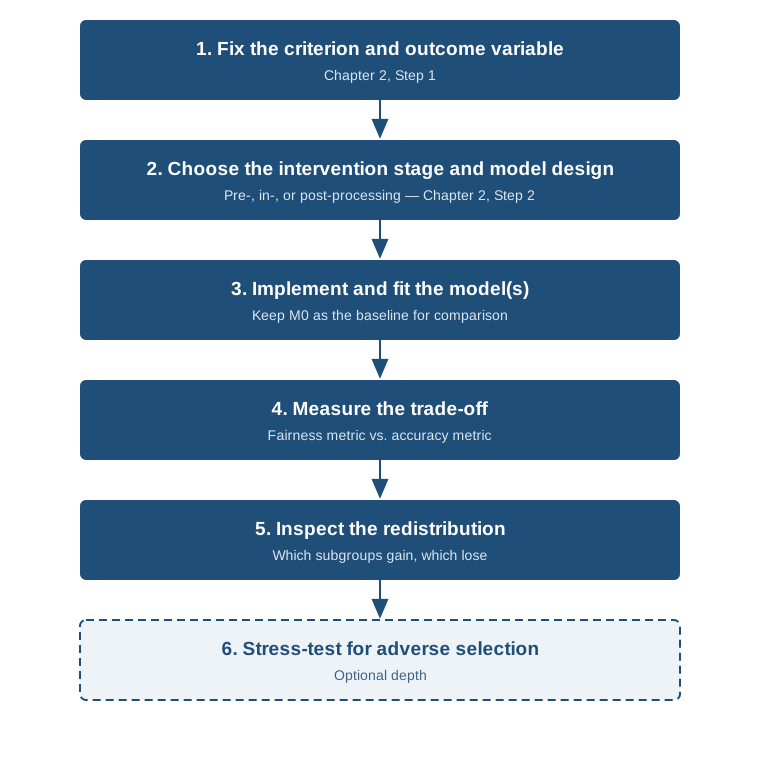
The workflow

1. Fix the criterion and the outcome variable (Ch 2, Step 1)
2. Choose the intervention stage, pre/in/post-processing (Ch 2, Step 2)
3. Implement and fit, keeping M0 as baseline
4. Measure the trade-off, fairness metric vs. accuracy metric
5. Inspect the redistribution, who gains, who loses

Same sequence, regardless of domain.

The workflow, visualised

Case study: fair pricing for motor insurance

• 100,000 French motor third-party-liability policies
• Response: pure premium = frequency × severity
• Protected attribute: Gender
• Legitimate: Age, Bonus, vehicle group, Density, Value
• Non-legitimate: InsuranceScore, a constructed credit-score-style proxy

Pure premium is roughly the average expected claims cost per policy. Frequency means how often a policyholder claims, severity means the average cost per claim. Third-party-liability covers damage or injury the policyholder causes to others, not their own vehicle. Bonus is a no-claims discount level, sometimes called bonus-malus, where lower means fewer past claims.

InsuranceScore stands in for a proxy-rich factor: retains predictive value, may correlate with gender, attracts stricter fairness scrutiny. Also serves a practical purpose. The disparate-impact remover needs continuous inputs, so summarising categorical proxies into one score makes debiasing feasible under MCDP.

The five models

Model	Criterion	Approach
M0	Baseline	Full model, includes Gender
MU	FTU (Fairness Through Unawareness)	Gender removed
MDP	Demographic parity	All predictors debiased
MCDP	Conditional DP	Only InsuranceScore debiased
MC	CPV (Controlling for Protected Variable)	Full model, average over Gender at scoring

Each fitted with GLM (Poisson frequency + Gamma severity) and XGBoost.

💬 Discuss (3 min)

If your organisation had to deploy one of these five designs tomorrow —

which would you pick, and why?

Part 2 — Fitting the models

Pre-processing: the disparate-impact remover

For MDP and MCDP, adjust continuous predictor distributions so they no longer depend on Gender, preserving overall shape.

di_data <- disparate_impact_remover(
  data = data_for_di, protected = as.factor(data$Gender),
  features_to_transform = features_to_transform, lambda = 1
)

• MDP: apply to all predictors
• MCDP: apply only to InsuranceScore

GLM frequency–severity framework

\text{Pure Premium} = \text{Claim Frequency} \times \text{Claim Severity}

• Frequency: Poisson GLM, log link, exposure offset
• Severity: Gamma GLM, log link, claims-only data

Age entered as a flexible function (\text{Age}, \log(\text{Age}), \text{Age}^2, \text{Age}^3, \text{Age}^4).

Exposure is the length of time, in days, a policy was active and at risk of a claim, used to normalise claim counts. XGBoost fitted the same way with the same predictor set, count:poisson objective for frequency. All models proportionally scaled so total predicted premium matches GLM MU’s portfolio total (the sum of predicted premiums across all policies). This focuses comparison on redistribution, not portfolio-level differences.

Part 3 — Results

Fairness metrics

Disparate Impact Ratio (DIR): \dfrac{\mathbb{E}(\hat{Y} \mid X_P = b)}{\mathbb{E}(\hat{Y} \mid X_P = a)}

• Close to 1 = similar average premiums across groups
• Four-fifths rule: expect 0.8 – 1.25

RMSE (accuracy, lower = better)

The Disparate Impact Ratio is how we check demographic parity here, the idea that predicted outcomes should not differ, on average, by protected group.

Fairness–accuracy trade-off

Dashed line = DIR of 1 (most fair). Dotted lines = the four-fifths band. Points further left (lower RMSE) are more accurate. M0 sits well outside the fair band with the worst accuracy. MDP, MCDP, MC all land inside it with only a small accuracy cost. Key finding: MCDP and MC achieve DIR close to 1 with only modest accuracy loss relative to M0.

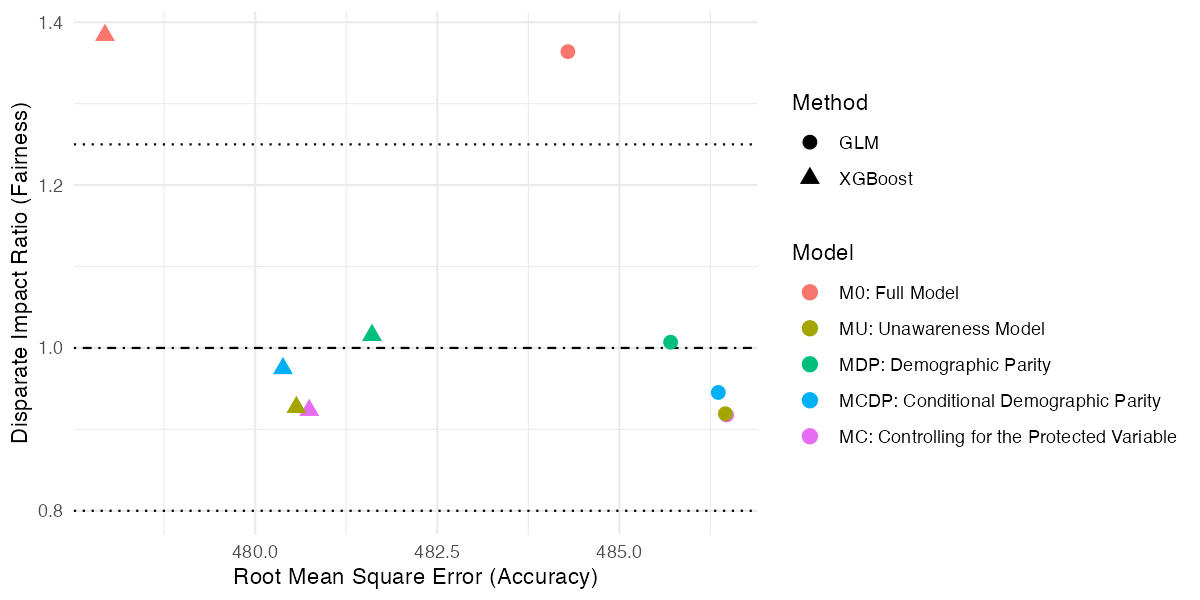
Reading the plot

• M0 (red): most accurate, most unfair, above the four-fifths ceiling (DIR 1.36)
• MU (olive): moves enough to land inside the fair band, but overshoots past DIR = 1 (to 0.92), reversing which gender pays more
• MDP, MCDP, MC: land inside the fair band, small accuracy cost
• XGBoost (▲) retains most of its edge over GLM (●) at every fairness level

The cost of fairness here is real, but small.

💬 Discuss (3 min)

Removing Gender doesn’t just shrink the gender gap in MU. It reverses which gender pays more.

What does that tell you about unawareness alone?

Break — 10 min

Part 4 — Premium redistribution

Who gains and who loses?

Compare each fair model to MU (the industry-standard benchmark):

\text{Relative Premium Difference}_{i} = \frac{\bar{Y}_{\text{model},i} - \bar{Y}_{\text{MU},i}}{\bar{Y}_{\text{MU},i}}

Positive = fair model charges more than MU · Negative = charges less

Premium redistribution by age and gender

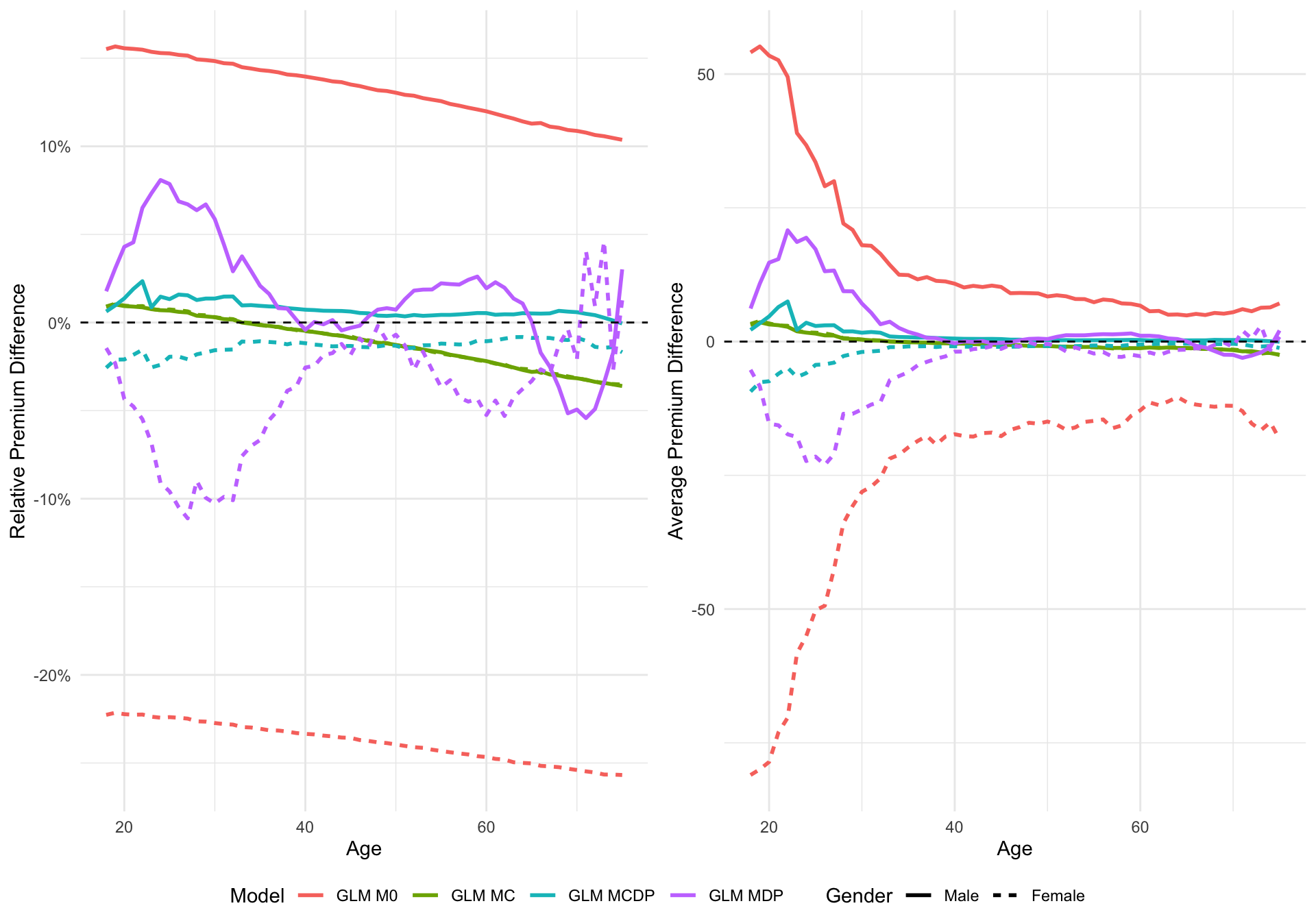
Reading the plot

• MDP: clearest transfer, raising the lower-charging group and lowering the higher-charging group across most ages
• MCDP: stays closest to MU, legitimate variables untouched, only the proxy is debiased
• MC: intermediate, reflecting only the gender coefficient in M0

The solidarity principle: stricter criteria imply more cross-subsidy between groups.

💬 Discuss (4 min)

MDP produces the largest transfer between groups.

Who would push back hardest against deploying MDP, and what would they say?

Part 5 — Case study: pretrial risk assessment (COMPAS)

The scenario

A US county is deciding whether to renew its contract for a pretrial risk-assessment tool that helps judges set bail and release conditions.

• Credited with reducing unnecessary pretrial detention
• An independent audit finds it over-flags Black defendants who do not reoffend
• The county’s Chief Public Defender must decide: does it meet a defensible fairness standard, and can it be corrected without becoming useless?

This mirrors the real ProPublica investigation into the actual COMPAS tool. Civil-rights advocates argue for scrapping it; the vendor and some judges argue it still outperforms unstructured human judgment.

From pricing to classification

Everything above is regression (continuous cost). This decision is binary: release/detain, flag/clear.

The M0/MU framework applies unchanged. Only the model type and metrics change.

• N = 5,278 defendants (2,103 Caucasian; 3,175 African-American)
• Response: two-year recidivism · Protected attribute: ethnicity
• Base rates already differ sharply: 39.1% vs 52.3%

Recidivism means being arrested for a new crime after release. Two-year recidivism here means within two years of release.

Fitting M0 and MU

m0 <- glm(Two_yr_Recidivism ~ Number_of_Priors + Age_Above_FourtyFive +
            Age_Below_TwentyFive + Female + Misdemeanor + ethnicity,
          data = compas_data, family = binomial)

mu <- glm(Two_yr_Recidivism ~ Number_of_Priors + Age_Above_FourtyFive +
            Age_Below_TwentyFive + Female + Misdemeanor,
          data = compas_data, family = binomial)

M0 includes ethnicity directly. MU removes it, mirroring the real COMPAS tool.

Three fairness checks

Criterion	M0 disparity ratio	MU disparity ratio
Demographic parity	2.11	1.94
Equal opportunity / TPR gap	1.75	1.67
Predictive rate parity / precision gap	1.11	1.15

Unawareness barely moves anything. MU costs almost no accuracy (66.5% vs 66.8%). Every disparity ratio survives nearly unchanged.

A defendant counts as flagged high-risk when the model’s predicted probability of reoffending is above the cutoff, 0.5 here. An African-American defendant who will NOT reoffend is flagged high-risk roughly twice as often as a Caucasian defendant who will not reoffend (FPR: 33.0% vs 17.2% under MU), the same qualitative finding ProPublica reported for the real tool, replicated here on a simple logistic regression.

Why do the three checks disagree?

Important

Demographic parity ignores the true outcome. It fully reflects the base-rate gap (39.1% vs 52.3%) plus any model unfairness. Precision conditions on the prediction, partly absorbing that same gap.

This is Chapter 2’s impossibility result, on real data: separation and sufficiency can’t both hold when base rates differ. Choosing a criterion is choosing how much of the base-rate difference counts as “unfairness” vs. “signal.”

💬 Discuss (4 min)

The three checks disagree sharply on how bad COMPAS’s disparity is.

If you were a judge deciding whether to use this tool, which check would you trust most, and why?

Post-processing: roc_pivot()

This reject-option correction relabels predictions within theta of the cutoff, giving the disadvantaged group’s borderline cases the benefit of the doubt.

• Mechanism: mirrors borderline probabilities across the cutoff (p \to 2\cdot\text{cutoff} - p) — a privileged borderline “favourable” case flips to unfavourable; a disadvantaged borderline “unfavourable” case flips to favourable. Confident predictions outside the band are untouched.

theta	Accuracy	Demographic parity	TPR gap	Precision gap
0 (MU)	66.5%	1.94	1.67	1.15
0.05	65.7%	1.13	1.11	1.31
0.10	62.8%	0.63	0.69	1.45
0.20	56.8%	0.23	0.30	1.73

Reading the trade-off

Important

Pushing demographic parity and the TPR gap toward 1 does not leave precision alone — it actively worsens it (1.15 → 1.73). Past theta ≈ 0.10, the correction overshoots and reverses the disparity, at a steep accuracy cost.

No theta satisfies all three checks at once, because none exists while base rates differ. Post-processing lets you choose where on the curve to sit. It doesn’t let you escape the curve.

💬 Discuss (5 min) — wrap-up

Post-processing dials fairness up on one criterion, always at the cost of another.

If you had to pick a theta for a real deployed system, how would you decide where to stop?

Summary

• All four designs work on real data with modest accuracy loss, and the same workflow transfers to classification (COMPAS)
• Model choice should follow the regulatory criterion, not modelling convenience
• MDP: strongest group fairness, largest redistribution. MCDP: more targeted
• Unawareness (MU) is rarely sufficient alone
• Post-processing can hit one criterion, never all three at once

Recommended reading

• Xin and Huang (2024), the five model designs and trade-off analysis
• Barocas et al. (2023), Ch 2–3 (Classification, Regression), fairmlbook.org
• Kozodoi and V. Varga (2021); Kamiran et al. (2012), the R packages and methods used today

Next class

Chapter 4 — Explainability Principles

Bring one prediction from today’s models you’d want explained to a policyholder.

Barocas, Solon, Moritz Hardt, and Arvind Narayanan. 2023. Fairness and Machine Learning: Limitations and Opportunities. MIT Press. https://fairmlbook.org.

Kamiran, Faisal, Asim Karim, and Xiangliang Zhang. 2012. “Decision Theory for Discrimination-Aware Classification.” 2012 IEEE 12th International Conference on Data Mining, 924–29.

Kozodoi, Nikita, and Tibor V. Varga. 2021. Fairness: Algorithmic Fairness Metrics. https://CRAN.R-project.org/package=fairness.

Xin, Xi, and Fei Huang. 2024. “Antidiscrimination Insurance Pricing: Regulations, Fairness Criteria, and Models.” North American Actuarial Journal 28 (2): 285–319.