Explainability Principles

Slides — Chapter 4

Fei Huang, UNSW Sydney

Table of contents

• What is explainability?
• Taxonomy of methods
• PFI & PDP
• Break — 10 min
• SHAP & LIME
• Validation, communication & regulation

Today’s roadmap

2-hour session, five parts, five discussion breaks

Time	Part
0:00 – 0:30	What is explainability? Goals & stakeholders
0:30 – 0:50	Taxonomy of methods + explainable models
0:50 – 1:10	PFI & PDP
1:10 – 1:20	Break
1:20 – 1:45	SHAP & LIME
1:45 – 2:00	Validation, communication, LLMs, summary

Full detail in Lecture-Explainability-Principles.qmd. This chapter is dense. Pace deliberately, and use the discussion breaks to let concepts land before adding the next layer.

Learning objectives

• Define explainability, and recognise interpretability/transparency as closely related, often-interchangeable terms
• Explain why explainability matters in high-stakes domains
• Map stakeholder needs to explanation types
• Classify methods along the key taxonomic dimensions

What is explainability?

Why this matters: the toeslagenaffaire

2013–2019: a Dutch tax-authority algorithm flagged ~26,000 families for childcare-benefit fraud, weighting dual nationality as a risk factor.

Families couldn’t get a clear account of why they were flagged. Neither could the courts reviewing their cases.

Result: forced repayments, over 1,000 children removed from their homes, the Dutch government’s resignation (Jan 2021) (Amnesty International 2021).

The point isn’t that the algorithm was biased (though it was). It’s that nobody, not the family, not a caseworker, not a court, could get a clear, checkable account of why. That gap between a model’s output and a human’s ability to understand and contest it is what this chapter is about.

Core definitions

Explainability: converting a model’s internal logic into a form a specific audience can understand, for a specific purpose. A model is explainable to the degree a person can understand the cause of its decision (Biran and Cotton 2017).

Interpretability is often used for the same idea. Transparency sometimes means understanding a model’s structure directly, as opposed to a post-hoc explanation built after training.

This course won’t police the boundary sharply. The key question is always: for whom, about what, for what purpose?

Why does it matter?

Reason	Why
Human learning	Update mental models when outcomes surprise
Safety & testing	Confidence the model behaves correctly
Bias detection	A debugging tool for discriminatory patterns
Social acceptance	Trust and legitimacy
Auditing	Decisions must be visible to be evaluated
Right to explanation	GDPR, ASIC, EU AI Act mandate it

When is it not required?

• Low stakes — no significant consequences from errors
• Well-established & tested — standard actuarial (insurance risk-pricing) tables, validated clinical rules
• Transparency enables gaming — fraud scoring systems

Most domains this course covers — lending, hiring, healthcare, insurance — are high-stakes by default. Explainability is generally expected.

💬 Discuss (3 min)

Think of a low-stakes automated decision you’d be fine having explained by a black box.

What made it low-stakes?

💬 Which is the wolf?

What features are you actually using to decide?

Left: a wolf. Right: a Siberian husky (bred to resemble wolves). Most people separate them on facial and body proportions, not the background. The risk in a classifier is when it doesn’t use those features. In the original example this course draws on, a wolf-vs-husky image classifier turned out to rely on background snow, not the animal, because most training-set wolf photos happened to be snowy. Photograph a husky in snow and the model calls it a wolf. Test-set accuracy looked fine; the model had learned the wrong thing.

Three goals of explainability

1. Improving the model — catch unintended patterns (the wolf/husky snow shortcut; a proxy variable slipping through undetected)
2. Justifying predictions — different stakeholders need different verification
3. Discovering insights — relationships useful for product design, pricing, science

Insurance analogue: using a proxy (a feature that indirectly stands in for another) for a protected attribute (a legally protected characteristic such as race or gender) without detection.

Characteristics of good explanations

Principle	Implication
Contrastive	“Why this, not that?” beats a full causal chain
Selective	1–2 reasons accepted, even with many contributors
Social	Varies by audience
Abnormality focus	Rare features make stronger explanations
Consistent with beliefs	Persuasive — but watch confirmation bias
Faithful	Must truthfully reflect model behaviour

Who needs explanations?

Stakeholder	Need
Model creators	Debugging, feature engineering
Operators (insurers, banks, hospitals)	Compliance, governance, sign-off
Executors (underwriters, clinicians)	Verify outputs before acting
Decision subjects	Understand why
Auditors	Validate fairness, accuracy

Case Study: stakeholder mapping in insurance

Actuary → “does the model behave sensibly?” (global). Underwriter → “why this premium?” (local). Customer → “why did my premium rise?” (local, plain language). Regulator → “is this fair?” (global, statistical).

Underwriter: the insurance professional who decides whether to accept a risk and sets its price. Actuary: the professional who builds, prices, and validates the risk models and signs off on them. Premium: the price a customer pays for insurance cover.

Taxonomy of methods

Two primary categories

Explainability by design: GLM (generalised linear model), GAM (generalised additive model), decision trees, RuleFit (rules combined with a linear model), all inherently interpretable

Post-hoc: applied after training to explain an existing model (SHAP, PDP, LIME)

This choice is made before modelling, not as an afterthought.

Three independent axes

Dimension	Values
Origin	Intrinsic (GLM, tree) vs. post-hoc (SHAP, PDP, LIME)
Applicability	Model-agnostic (SHAP, PDP, PFI) vs. model-specific (TreeSHAP, GLM coefficients)
Scope	Global (PFI, PDP) vs. local (single SHAP value, LIME)

Independent axes, not a hierarchy. TreeSHAP is post-hoc + model-specific. A single SHAP value is local, and its mean absolute value is global.

💬 Discuss (3 min)

Pick a method you’ve heard of, even vaguely.

Where does it sit on the three axes (intrinsic/post-hoc, agnostic/specific, global/local)?

Explainable models, briefly

GLM: \log \mathbb{E}[Y_i] = \beta_0 + \beta_1 x_{i1} + \cdots. Each coefficient has a direct reading — this chapter’s own insurance frequency model gives Age a coefficient of -0.0049, a 0.5% drop in expected claim frequency per extra year, holding other factors fixed

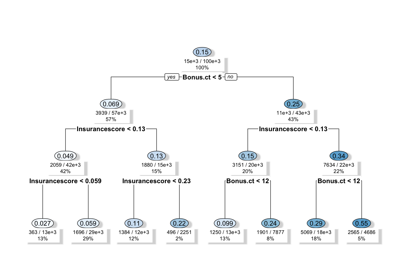
Decision trees: rectangular partitions, visualisable, but unstable and prone to overfitting

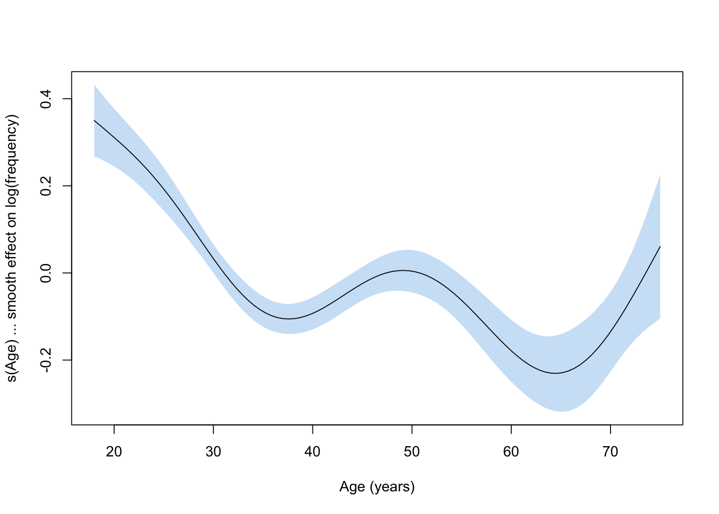
GAMs: g(\mathbb{E}[Y]) = \beta_0 + f_1(x_1) + \cdots, smooth functions, more flexible than GLM, still plottable

GLMs are the standard in regulated scoring settings precisely because they’re intrinsically interpretable. Neural additive models (NAMs) extend the additive idea to deep learning.

Decision tree, a real example

Fit directly on the insurance frequency data (Bonus, then Insurancescore splits). Every leaf’s predicted frequency is readable straight off the diagram, no equation needed, but three splits already start to feel unstable: a slightly different training sample could easily pick different cut points.

GAM, a real example

The smooth effect of Age on log(claim frequency), fitted on the same data. A GLM’s single Age coefficient could only draw a straight line through this; the GAM’s spline captures the dip through the 30s-50s and the late-life uptick a straight line would average away.

The accuracy–explainability trade-off

More flexible models (boosting, neural nets) → more accurate, less explainable.

Real, but not fixed. GAMs and constrained boosting narrow the gap. Post-hoc explanation of a black box is always an approximation, never fully faithful.

Boosting combines many simple models, often shallow decision trees, into one strong model (e.g. XGBoost, LightGBM).

PFI & PDP

Permutation Feature Importance

“A feature is important if shuffling its values increases model error.” (Molnar 2025)

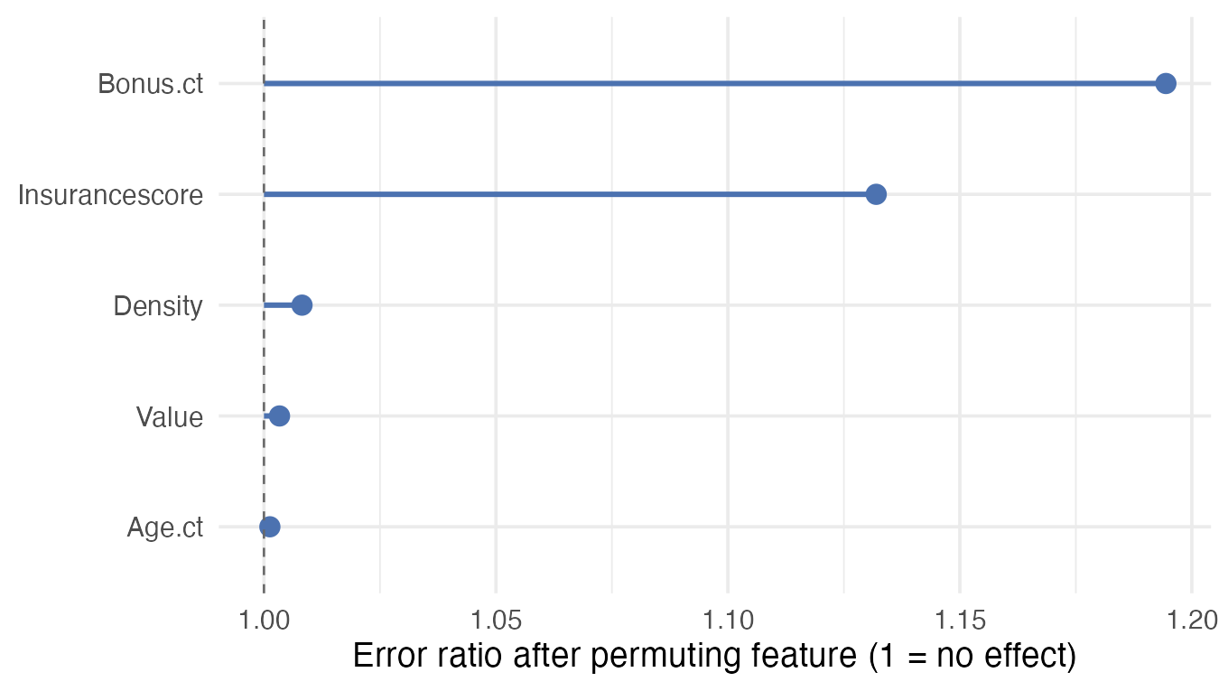
Algorithm: baseline error → shuffle one column → re-score (no retraining) → importance = error change. Repeat per feature.

Strength: captures interactions, no retraining. Limitation: unrealistic combinations when features are correlated.

Case Study: reading a PFI ranking

In a motor pricing model, Age and Bonus (a driver’s no-claims discount level) dominate (expected). InsuranceScore (a non-legitimate proxy) contributes significantly too, a signal that fairness scrutiny is needed.

PFI, a real example

Same insurance frequency model. Bonus and Insurancescore are the only two features whose permutation meaningfully increases error (ratio > 1); Density, Value, and Age barely move it. Insurancescore showing up here, despite being the non-legitimate proxy, is exactly the fairness-scrutiny signal the case study above describes.

Partial Dependence Plots

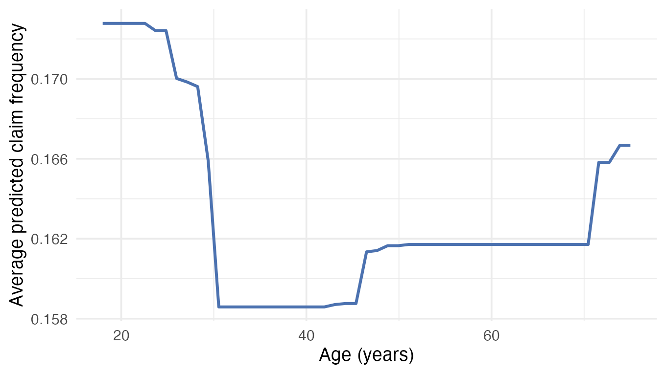
Fix a feature to a value, average predictions across all observations, repeat across the range.

\hat{f}_j(x_j) \approx \frac{1}{n}\sum_{i=1}^n \hat{f}(x_j, x_{-j}^{(i)})

Limitation: assumes feature independence, and extrapolates into unrealistic combinations when features correlate. Use ALE instead when they do.

PDP shows direction, shape, magnitude. Admits a causal reading only under additional causal assumptions, not automatically. Two-feature PDPs can reveal possible interaction, but confirming it needs the H-statistic or SHAP interaction values (Chapter 5).

PDP, a real example

Age’s PDP on the same insurance frequency model, fit with a flexible model so the curve isn’t forced to be a straight line. High for young drivers, a steep drop through the late 20s, flat through midlife, then a rise after about 65, a shape a GLM coefficient could not represent directly, but the PDP makes visible regardless of model type.

PD plots can be gamed

Xin et al. (2025) show the two limitations above aren’t just theoretical: a black-box model can be built so its real predictions barely change, while its PD plot for a protected or proxy variable is engineered to look flat.

Validated on real insurance and COMPAS data. A flat PD plot is not proof of fairness.

The attack exploits exactly the extrapolation and heterogeneous-averaging weaknesses just covered: it swaps in a decoy output only for the sparse, extrapolation-only region the averaging step depends on, so real-world predictions barely move. Relevant to insurance specifically because PD plots are exactly what the NAIC Model Review Manual asks insurers to submit for this kind of check.

💬 Discuss (3 min)

Name two correlated features in a domain you know.

What would a PDP get wrong there?

Break — 10 min

SHAP & LIME

SHAP

Assigns each feature a Shapley value (a concept from cooperative game theory for fairly splitting credit among contributors), its average contribution across all possible feature-subset orderings (Lundberg and Lee 2017).

g(z') = \phi_0 + \sum_{j=1}^p \phi_j z_j'

The only method satisfying local accuracy, missingness, and consistency simultaneously.

KernelSHAP: model-agnostic, slower. TreeSHAP: exact and fast for tree models, the default for XGBoost/LightGBM across domains.

Reading a SHAP waterfall

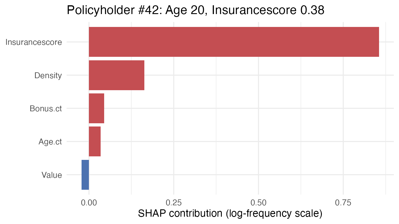
Case Study: SHAP waterfall for a premium

For one policyholder (the insurance customer), age (young) pushes the prediction up, while bonus (strong no-claims record) pushes it down. Sum of pushes/pulls from the baseline = this individual’s deviation.

“Your premium is higher than average mainly because of your age and driving history.”

This is the natural format for a customer-facing explanation. The same structure works for a declined loan or a clinical risk score.

SHAP, a real example

One policyholder from the insurance frequency model (young driver, high Insurancescore). Insurancescore alone accounts for most of the upward push, Density adds a little more, Bonus and Age push in small opposite directions, Value pulls it down slightly. A genuine SHAP decomposition, not a mock-up.

LIME

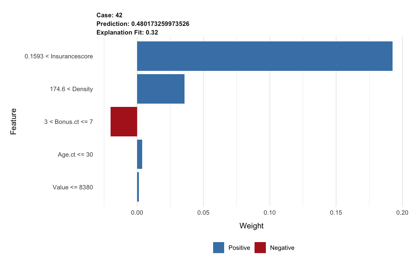
Fits a simple, interpretable model in the local neighbourhood around one prediction. Even a complex model may look linear nearby.

Strength: works for tabular, text, image data. Limitation: unstable. Nearby points can yield very different explanations, and neighbourhood-width choice matters a lot.

LIME, a real example

Same policyholder as the SHAP example, explained locally by LIME instead. Notice the “Explanation Fit” of 0.32, a low fidelity score, exactly the instability caveat from the previous slide: LIME’s local surrogate is only a partial approximation of what the real model is doing at this point.

SHAP vs LIME

	SHAP	LIME
Basis	Game theory	Local surrogate
Consistency	Guaranteed	Not guaranteed
Stability	High (TreeSHAP)	Low
Best for	Production, tree models	Quick exploration

💬 Discuss (4 min)

A SHAP value for “Age” is high in a claims model. A colleague says: “so age causes higher claims.”

What’s wrong with that leap?

Validation, communication & regulation

Are explanations faithful?

An explanation can be plausible without being accurate.

• Sanity check: match domain knowledge?
• Consistency: similar individuals, similar explanations?
• Simulation test: perturb a feature, does its SHAP value move as expected?
• Adversarial check: could a biased model be designed to look fair? (Slack et al. 2020)

Common pitfalls

1. Explanation ≠ causation — high SHAP for Age means the model uses Age, not that Age causes the outcome
2. Global ≠ local — globally-unimportant feature can dominate one prediction
3. Correlation blindness — PDP/KernelSHAP can extrapolate into unrealistic regions. ALE fixes this, but TreeSHAP does not automatically
4. LIME instability — never present one run as definitive
5. Confirmation bias — plausible-and-wrong explanations are persuasive too
6. A flat PD plot ≠ proof of fairness — PDP’s own weaknesses can be exploited to hide it (Xin et al. 2025)

Regulatory expectations

• EU AI Act: high-risk systems (credit, employment, insurance) must explain to affected individuals
• GDPR Art 22: automated decisions must be explainable and contestable
• China’s PIPL Art 24: right to an explanation, and to refuse a solely-automated decision (National People’s Congress (China) 2021); NFRA also names explainability as a required AI governance element (National Financial Regulatory Administration (China) 2026)
• Singapore’s MAS FEAT (Transparency): internal documentation plus meaningful explanations to affected customers (Monetary Authority of Singapore 2018)
• Sector rules add detail: ECOA/FCRA adverse-action notices, NYC Local Law 144 bias audits, APRA CPG 234

Explainability is becoming a compliance obligation, not just good practice.

Explainability for large language models

PDP/SHAP/LIME all assume a fixed feature set. An LLM has none — tokens in a variable-length prompt, billions of parameters.

Chain-of-thought is not a faithful explanation (Turpin et al. 2023): models shift answers toward a hidden biasing feature without ever mentioning it in their stated reasoning.

Mechanistic interpretability is the emerging alternative (Templeton et al. 2024), opening the model’s internals directly rather than trusting its self-report. Still a research frontier, not a routine audit tool.

💬 Discuss (5 min) — wrap-up

If chain-of-thought text isn’t a faithful explanation —

what should you actually tell a customer, when an LLM-assisted decision affects them?

Summary

• PFI: global ranking of what matters
• PDP: average marginal effect. Use ALE if correlated
• SHAP: principled, versatile, additive contributions
• LIME: local surrogate, quick but unstable
• Plausibility ≠ faithfulness. Communication must match the audience

Recommended reading

• Molnar (2025) — free textbook, christophm.github.io/interpretable-ml-book
• Lundberg and Lee (2017); Ribeiro et al. (2016) — original SHAP, LIME papers
• Xin et al. (2025) — manipulating PD plots to hide discrimination
• Turpin et al. (2023); Templeton et al. (2024) — explainability for LLMs

Next class

Chapter 5 — Explainability Practice

Bring a laptop with Python installed. We’ll compute PFI, PDP, SHAP on a real pricing model.

Amnesty International. 2021. Xenophobic Machines: Discrimination Through Unregulated Use of Algorithms in the Dutch Childcare Benefits Scandal. Amnesty International. https://www.amnesty.org/en/documents/eur35/4686/2021/en/.

Biran, Or, and Courtenay Cotton. 2017. “Explanation and Justification in Machine Learning: A Survey.” IJCAI-17 Workshop on Explainable AI (XAI).

Lundberg, Scott M, and Su-In Lee. 2017. “A Unified Approach to Interpreting Model Predictions.” Advances in Neural Information Processing Systems 30.

Molnar, Christoph. 2025. Interpretable Machine Learning: A Guide for Making Black Box Models Explainable. 3rd ed. https://christophm.github.io/interpretable-ml-book/.

Monetary Authority of Singapore. 2018. “Principles to Promote Fairness, Ethics, Accountability and Transparency (FEAT) in the Use of Artificial Intelligence and Data Analytics in Singapore’s Financial Sector.” https://www.mas.gov.sg/publications/monographs-or-information-paper/2018/feat.

National Financial Regulatory Administration (China). 2026. Guidance on the Safe Development and Application of Artificial Intelligence in the Banking and Insurance Sectors (关于银行业保险业人工智能安全开发应用的指导意见, Jin Fa [2026] No. 8). https://www.nfra.gov.cn/cn/view/pages/governmentDetail.html?docId=1261784&generaltype=1.

National People’s Congress (China). 2021. Personal Information Protection Law of the People’s Republic of China (中华人民共和国个人信息保护法). http://www.npc.gov.cn/npc/c2/c30834/202108/t20210820_313088.html.

Ribeiro, Marco Tulio, Sameer Singh, and Carlos Guestrin. 2016. “Why Should i Trust You?: Explaining the Predictions of Any Classifier.” Proceedings of the 22nd ACM SIGKDD International Conference on Knowledge Discovery and Data Mining, 1135–44.

Slack, Dylan, Sophie Hilgard, Emily Jia, Sameer Singh, and Himabindu Lakkaraju. 2020. “Fooling LIME and SHAP: Adversarial Attacks on Post Hoc Explanation Methods.” Proceedings of the AAAI/ACM Conference on AI, Ethics, and Society, 180–86.

Templeton, Adly, Tom Conerly, Jonathan Marcus, et al. 2024. “Scaling Monosemanticity: Extracting Interpretable Features from Claude 3 Sonnet.” Transformer Circuits Thread. https://transformer-circuits.pub/2024/scaling-monosemanticity/index.html.

Turpin, Miles, Julian Michael, Ethan Perez, and Samuel R Bowman. 2023. “Language Models Don’t Always Say What They Think: Unfaithful Explanations in Chain-of-Thought Prompting.” Advances in Neural Information Processing Systems 36.

Xin, Xi, Giles Hooker, and Fei Huang. 2025. “Pitfalls in Machine Learning Interpretability: Manipulating Partial Dependence Plots to Hide Discrimination.” Insurance: Mathematics and Economics 125: 103135. https://doi.org/10.1016/j.insmatheco.2025.103135.