Explainability Practice

Slides — Chapter 5

Fei Huang, UNSW Sydney

Table of contents

• Motivation
• Part 1 — Setup
• Part 2 — Feature Importance
• Part 3 — Main effects: PDP and ALE
• Break — 10 min
• Part 4 — SHAP: global and local
• Part 5 — Interactions

Today’s roadmap

~2-hour session, hands-on, with five parts and five discussion breaks

Time	Part
0:00 – 0:10	Motivation: why interpretability, regulatory context
0:10 – 0:25	Setup, workflow and case study
0:25 – 0:50	Feature importance
0:50 – 1:15	Main effects, PDP and ALE
1:15 – 1:25	Break
1:25 – 1:55	SHAP, global and local
1:55 – 2:10	Interactions and summary

Full Python walkthrough lives in Lecture-Explainability-Practice.qmd. Bring it up on a second screen for the live coding. These slides carry the workflow, key plots, and discussion.

Learning objectives

• Operationalise post-hoc explainability end-to-end: importance → PDP/ALE → SHAP → interactions
• Interpret global variable importance and its limitations
• Use PDP and ALE to see predictor–prediction relationships
• Interpret SHAP values, globally and for one prediction
• Detect interactions with the H-statistic and SHAP interaction values

Motivation

💬 Discuss (2 min)

AI adoption across industries, including insurance, has led to widespread use of complex black-box models.

What are the benefits, and the potential risks, of that shift?

Benefits and risks of AI

• Benefits: enhanced efficiency and accuracy
• Risks: lack of transparency and interpretability

Adapted from Huang, “Why You Should Not Trust Interpretations in Machine Learning: Adversarial Attacks on Partial Dependence Plots” (All Actuaries Summit 2024), joint work with Xi Xin and Giles Hooker — the same paper behind the PDP manipulation case study in Chapter 4.

Why do we need interpretations?

Before the list: what would you say?

1. Transparency and explainability: explain how the model makes decisions to consumers, regulators, and managers, and build trust
   • Understand feature importance
   • Understand input–output relationships (main effects)
   • Identify and visualise interaction effects
   • Answer why, not just what — causality
2. Fairness: avoid discrimination and bias
3. Privacy: ensure sensitive information is protected
4. Model validation and robustness checks

Regulatory background on interpretability

Interpretability, explainability, and transparency are recurring requirements across AI principle documents:

• Stanford Human-Centered AI (HAI): a Jan. 2022 White Paper supporting the White House OSTP’s AI Bill of Rights
• Australia’s AI Ethics Principles
• EU GDPR (Regulation (EU) 2016/679 of the European Parliament and of the Council (General Data Protection Regulation) 2016): a “right to explanation”
  • Whether this right actually exists under the GDPR is itself debated (Wachter et al. 2017; Bordt et al. 2022)
• China’s Personal Information Protection Law, Article 24 (National People’s Congress (China) 2021): automated decisions must be transparent and their results fair; also grants a right to explanation

Insurance regulatory example: NAIC

• NAIC’s 2022 Predictive Models White Paper (National Association of Insurance Commissioners 2022) extended rate-filing review beyond GLMs to tree-based models (random forests, gradient boosting)
• Section B.3.d requires insurers to:
  • Obtain plots describing the relationship between each predictor variable and the target variable
  • Obtain a rational explanation for the observed relationship

This is exactly the kind of check this chapter’s PDP/ALE section responds to, and — as Chapter 4’s case study shows — exactly the check a manipulated PD plot can be made to pass without genuinely fixing a discriminatory model. NAIC’s current Model Review Manual (National Association of Insurance Commissioners 2025), cited later in this chapter, supersedes this 2022 white paper but keeps the same underlying expectation.

Interpretation methods: the landscape

(Partially) interpretable / transparent models

• LM, GLM, GAM, decision trees (CART)

Global model-agnostic methods

• PD plots, ALE plots, feature interaction (H-statistic), functional decomposition, permutation feature importance

Local model-agnostic methods

• ICE curves, local surrogate models (LIME), SHAP, counterfactual explanations, scoped rules (anchors)

Taxonomy from Molnar (Molnar 2025). Interpretable models were Chapter 4’s territory. This chapter works through the bulk of the global and local model-agnostic toolkit: permutation importance, PD/ALE, and SHAP, the parts most established in insurance practice. LIME, counterfactual explanations, and anchors follow the same model-agnostic logic but aren’t covered here. Pause after each category and ask students for examples or where a method they already know would fit before revealing the next one.

Part 1 — Setup

The workflow

1. Fit an accurate model. Explainability describes, it doesn’t fix
2. Check global importance. Which predictors drive it overall?
3. Check main effects. PDP and ALE, shape of each relationship
4. Check individual predictions. Local SHAP
5. Check interactions. Where does the additive picture break down?
6. Validate and communicate

Same sequence for any tabular model, any domain.

Case study: insurance pricing

• 100,000 French motor TPL (third-party liability) policies (2009–2010), pg15training
• XGBoost models: claim frequency, claim severity, pure premium (Tweedie)
• Predictors: age, bonus-malus, vehicle type/value, occupation, density, and more

XGBoost is a gradient boosting algorithm: an ensemble of decision trees where each new tree corrects the errors of the previous ones. Claim frequency = how often claims occur per year a policy is in force. Claim severity = the average cost per claim. Pure premium = frequency times severity, the expected claim cost per policy. The Tweedie distribution models pure premium directly in one step because it handles a mix of exact zeros (no claim) and positive amounts. Bonus-malus = a no-claims discount/surcharge score, covered in more depth on the Age/Bonus slides.

Interpretation toolkit and regulatory expectations (NAIC model review, SOA guidance) are unusually mature in insurance, but the workflow applies to any tabular ML model used for a high-stakes decision: credit scoring, hiring, healthcare risk.

💬 Discuss (3 min)

The workflow is: fit → global importance → main effects → local explanations → interactions → validate/communicate.

Which step gets skipped most often under deadline pressure, and what’s the risk?

Part 2 — Feature Importance

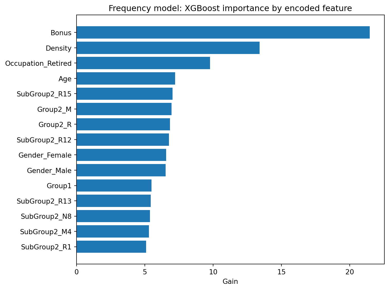
XGBoost built-in importance

Weight = split count, Gain = objective improvement, Cover = observations affected. We use gain because it is most directly tied to model fit.

Grouped importance — a pitfall

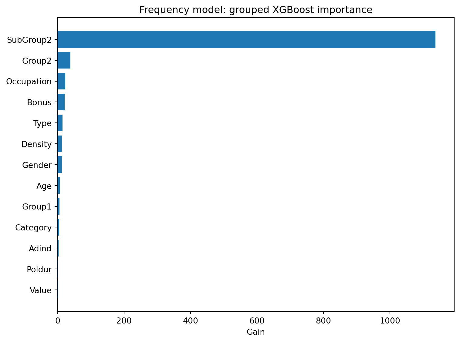
SubGroup2 dominates, partly an artifact. Many categories → many splitting points → inflated total gain. Bonus, Age, Density look less important after grouping, despite large individual encoded-feature gains.

Permutation feature importance

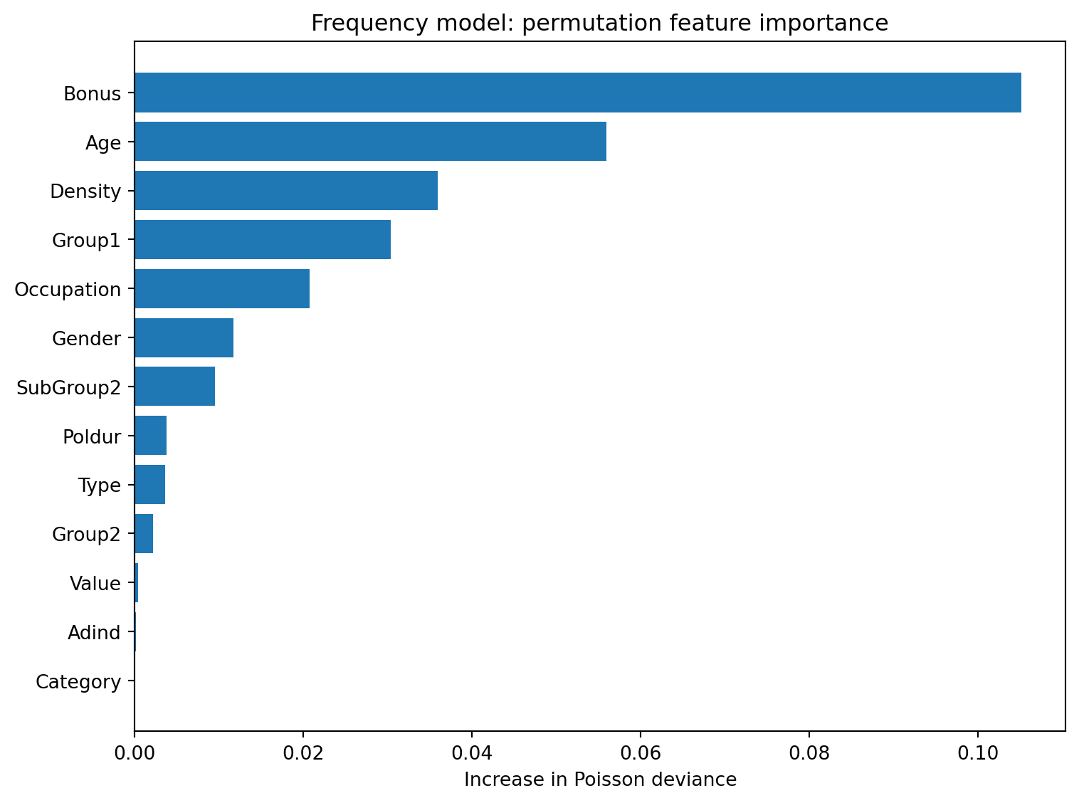
Model-agnostic (works the same way for any model type). Shuffle a column and measure the performance drop, no tree structure needed (Breiman 2001).

💬 Discuss (4 min)

Built-in gain says SubGroup2 dominates, partly a category-count artifact.

If you only had time for ONE importance method before a deadline, which would you trust more, and why?

Part 3 — Main effects: PDP and ALE

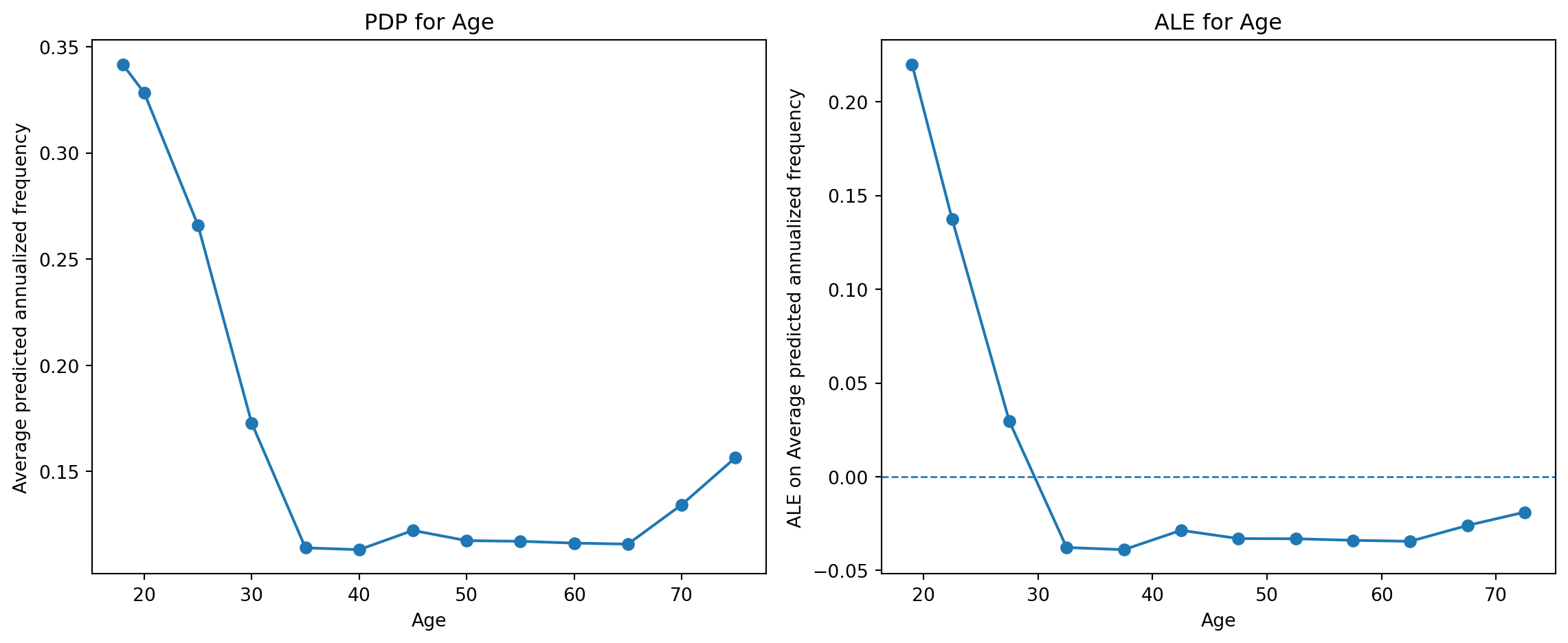
Age: PDP and ALE

Strong nonlinear effect. Very young drivers → much higher predicted frequency, declining rapidly to ~30, then stable. PDP and ALE closely agree. The effect is robust, not an artifact of correlation with other predictors.

PDP = partial dependence plot: the average predicted outcome as one predictor varies, holding everything else at its observed values. ALE = accumulated local effects plot: a similar idea, but built from local changes within the observed data, which makes it more robust when predictors are correlated.

Bonus: PDP and ALE

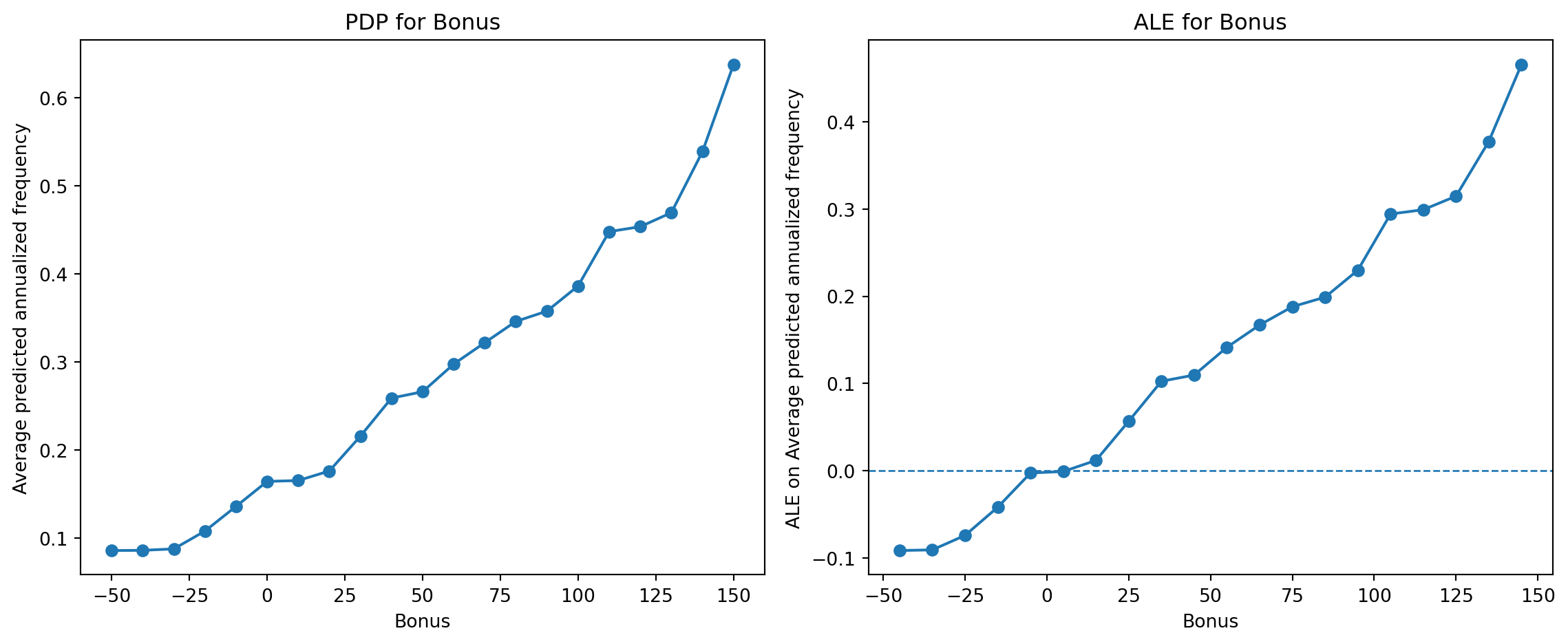
Approximately monotonic. Lower bonus (discount, clean history) → lower predicted frequency. Again PDP and ALE agree closely. The model has learned the expected relationship.

Break — 10 min

Part 4 — SHAP: global and local

Why SHAP?

PDP/ALE describe average effects. A regulator or policyholder asks. Why does this policy pay this premium?

SHAP bridges both, a portfolio-level ranking (consistent with PDP/ALE) and a decomposition of one prediction into feature contributions.

Important

Interpretation ≠ trustworthiness. SHAP and LIME can be adversarially manipulated to mask discriminatory behaviour (Slack et al. 2020). Pair explanations with validation and fairness assessment, not as proof on their own.

SHAP = SHapley Additive exPlanations, based on Shapley values from cooperative game theory. The idea: treat each feature as a “player” contributing to the prediction (the shared “payout”), and split credit among features fairly based on their average contribution across every possible order they could be added in.

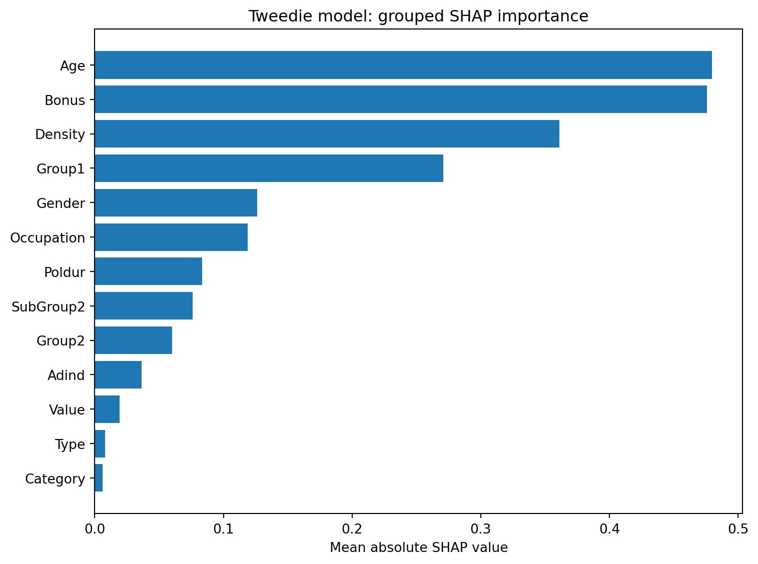
SHAP global: grouped importance

Ranks variables by mean |SHAP value|, similar spirit to PFI (permutation feature importance), based on actual contribution size.

SHAP global: beeswarm

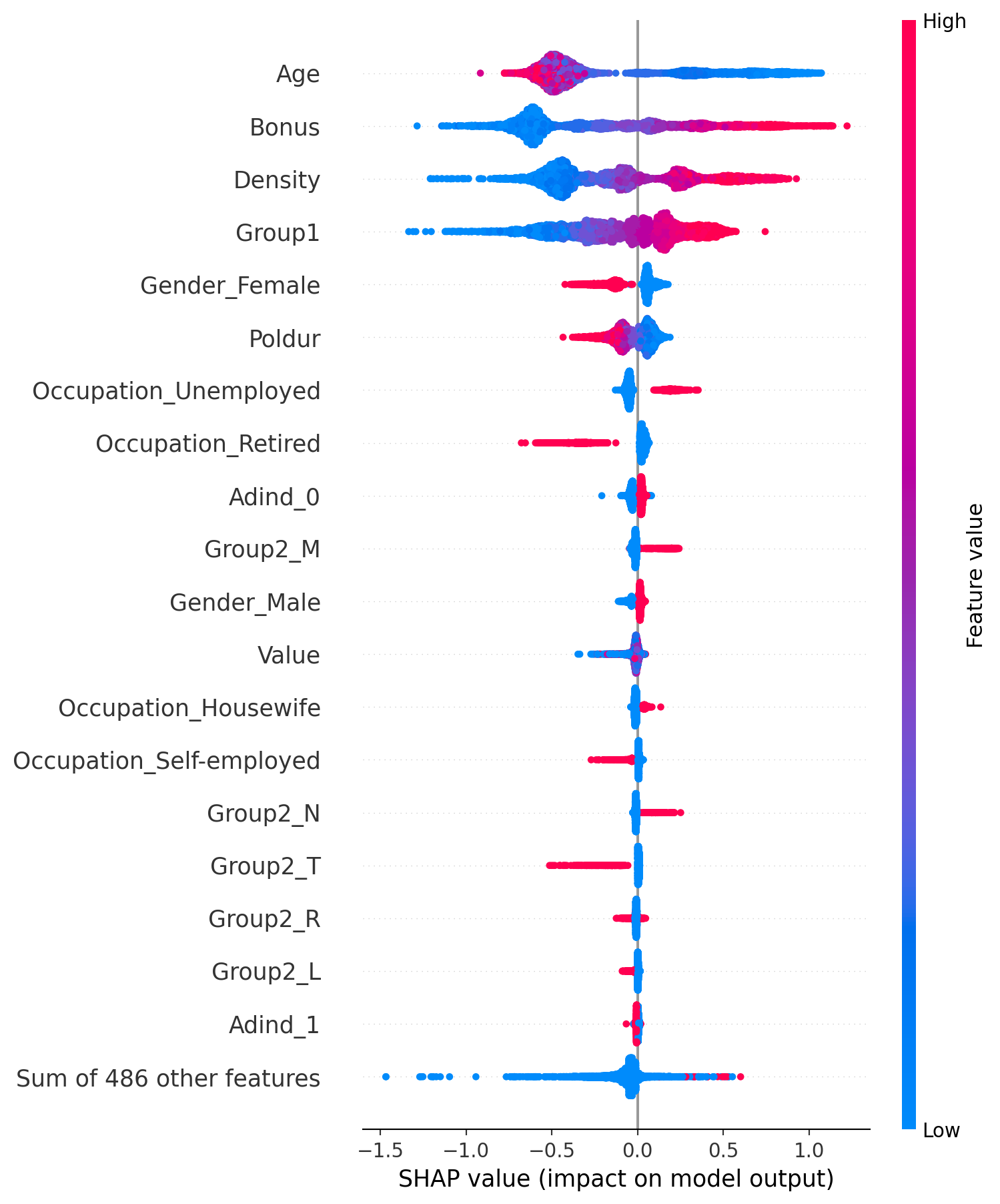
Each point = one policy × one feature. Position = SHAP value (pushes prediction up/down), and colour = feature value.

💬 Discuss (3 min)

The beeswarm shows both magnitude and direction, across every policy.

What can it tell you that a simple bar-chart importance ranking can’t?

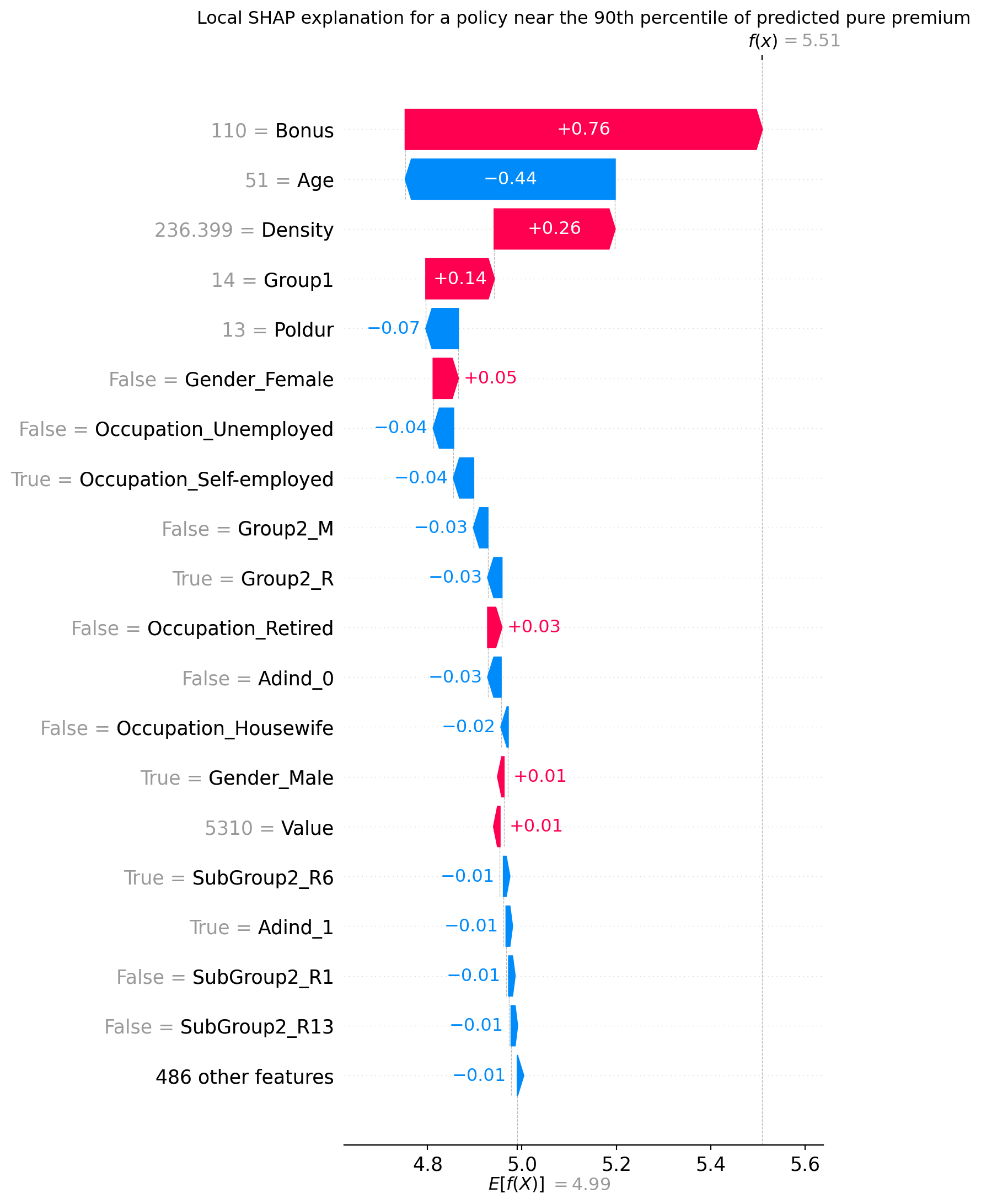
SHAP local: one policy’s premium

Policy near the 90th percentile of predicted pure premium. Largest positive contributions: Age = 20, Density = 236.4. Largest negative: Group1 = 5, Bonus = -10. Values are on the log scale (Tweedie model), so exponentiate to recover the pure premium. Broadly consistent with the global ranking. Age, Bonus, Density were already flagged as influential.

The natural format for a customer-facing explanation. For example, “your premium is higher mainly because of X and Y.”

Local what-if analysis

What would happen if one characteristic of this policy changed?

Vary one predictor at a time from the selected policy, holding the rest fixed at the median for continuous predictors and the most-common category otherwise.

Related to counterfactual explanations (finding the feature changes that would flip or substantially alter a prediction), but simpler. Not an optimal or realistic combined change, just a one-at-a-time sensitivity check.

Part 5 — Interactions

Why interactions matter

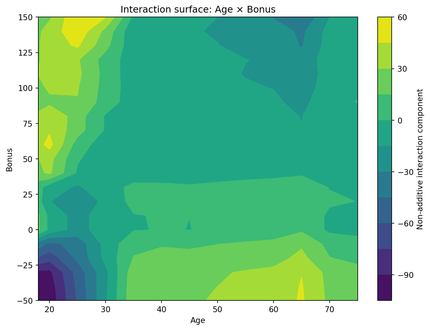
Everything so far treats each variable’s effect independently. But tree models routinely capture interactions. For example, the young-driver uplift might be amplified by a high bonus level.

Ignoring interactions can make single-variable summaries misleading.

Friedman’s H-statistic

Measures how far the joint effect of two variables departs from additive (Friedman and Popescu 2008). 0 = no interaction, closer to 1 = stronger.

SHAP interaction values

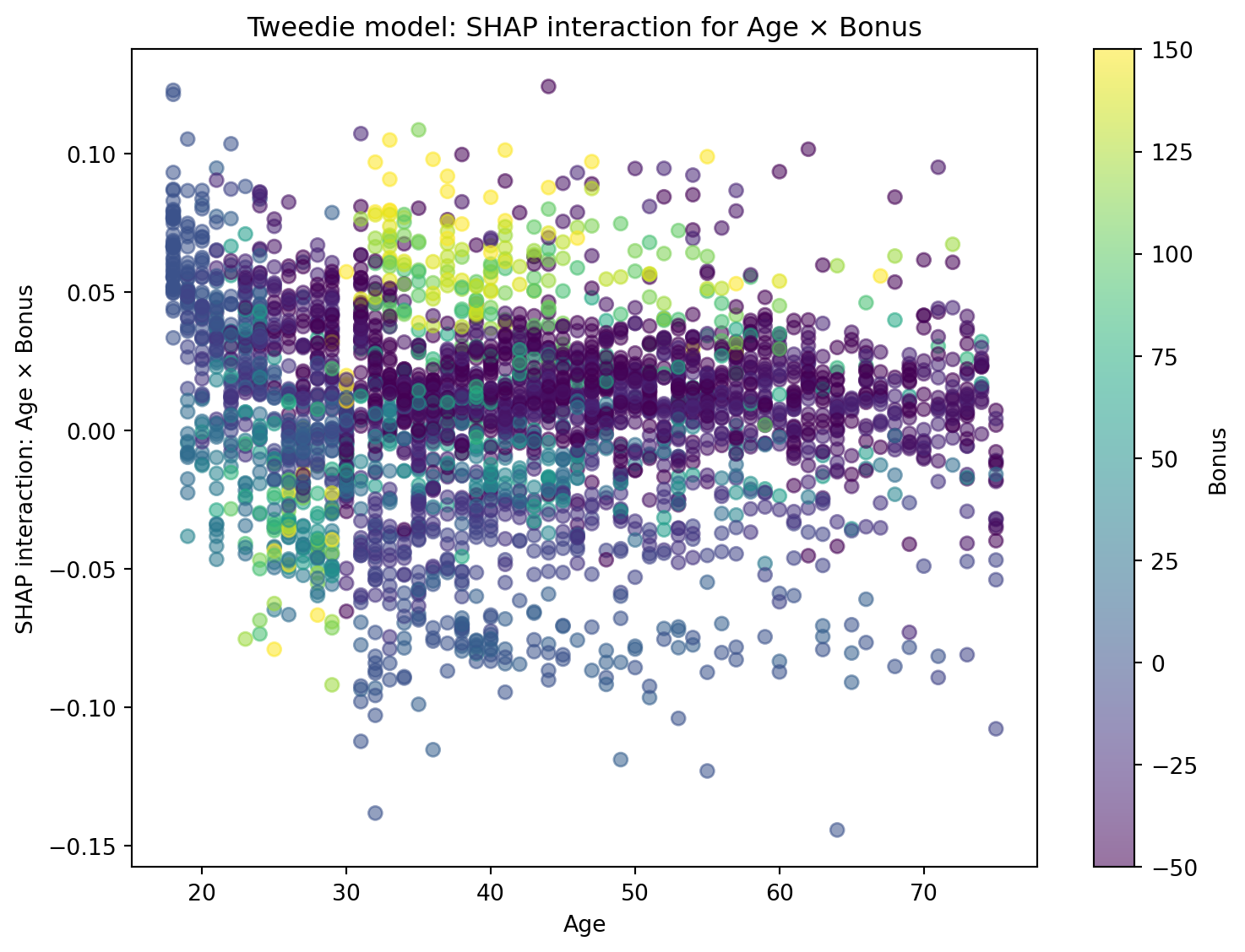
Same idea as the H-statistic, but allocated to individual predictions rather than a single portfolio-level number.

💬 Discuss (4 min)

If Age and Bonus interact strongly —

what’s wrong with explaining a policy’s premium using two separate, one-at-a-time SHAP contributions?

Summary

• Same workflow for any fitted tabular model, any domain
• No single method tells the whole story. Built-in vs. permutation importance can disagree, and PDP vs. ALE can disagree under correlation
• Interaction diagnostics show where the additive, one-variable-at-a-time picture breaks down
• Explanations are for an audience. Match the summary to who’s asking

💬 Discuss (5 min) — wrap-up

If you could only run two of today’s five methods on every model before deployment —

which two, and what would you be willing to miss?

Recommended reading

• Molnar (2025) — every method used today, in depth
• Baeder et al. (2021) — SOA report situating this toolkit in insurance practice
• Rudin (2019) — the case for interpretable-by-design over post-hoc explanation

Next class

Chapter 6 — Privacy Principles

Bring one example of personal data you’ve disclosed to a company recently, and think about what happened to it next.

Baeder, Larry, Peggy Brinkmann, and Eric Xu. 2021. Interpretable Machine Learning for Insurance: An Introduction with Examples. Society of Actuaries. https://www.soa.org/globalassets/assets/files/resources/research-report/2021/interpretable-machine-learning.pdf.

Bordt, Sebastian, Michèle Finck, Eric Raidl, and Ulrike von Luxburg. 2022. “Post-Hoc Explanations Fail to Achieve Their Purpose in Adversarial Contexts.” Proceedings of the 2022 ACM Conference on Fairness, Accountability, and Transparency, 891–905.

Breiman, Leo. 2001. “Random Forests.” Machine Learning 45 (1): 5–32.

Friedman, Jerome H., and Bogdan E. Popescu. 2008. “Predictive Learning via Rule Ensembles.” The Annals of Applied Statistics 2 (3): 916–54.

Molnar, Christoph. 2025. Interpretable Machine Learning: A Guide for Making Black Box Models Explainable. 3rd ed. https://christophm.github.io/interpretable-ml-book/.

National Association of Insurance Commissioners. 2022. Predictive Models White Paper. National Association of Insurance Commissioners.

National Association of Insurance Commissioners. 2025. Model Review Manual. National Association of Insurance Commissioners. https://content.naic.org/sites/default/files/inline-files/NAIC%20Model%20Review%20Manual__%20adopted%20by%20CASTF%2011.04.25.pdf.

National People’s Congress (China). 2021. Personal Information Protection Law of the People’s Republic of China (中华人民共和国个人信息保护法). http://www.npc.gov.cn/npc/c2/c30834/202108/t20210820_313088.html.

Regulation (EU) 2016/679 of the European Parliament and of the Council (General Data Protection Regulation) (2016).

Rudin, Cynthia. 2019. “Stop Explaining Black Box Machine Learning Models for High Stakes Decisions and Use Interpretable Models Instead.” Nature Machine Intelligence 1 (5): 206–15.

Slack, Dylan, Sophie Hilgard, Emily Jia, Sameer Singh, and Himabindu Lakkaraju. 2020. “Fooling LIME and SHAP: Adversarial Attacks on Post Hoc Explanation Methods.” Proceedings of the AAAI/ACM Conference on AI, Ethics, and Society, 180–86.

Wachter, Sandra, Brent Mittelstadt, and Luciano Floridi. 2017. “Why a Right to Explanation of Automated Decision-Making Does Not Exist in the General Data Protection Regulation.” International Data Privacy Law 7 (2): 76–99.