Privacy Practice

Slides — Chapter 7

Fei Huang, UNSW Sydney

Table of contents

• Part 1 — From principle to practice
• Part 2 — Re-identification risk
• Part 3 — k-Anonymity
• Break — 10 min
• Part 4 — Differential privacy
• Part 5 — Synthetic data
• Wrap-up

Today’s roadmap

2-hour-15-minute session, hands-on, with five parts and six discussion breaks

Time	Part
0:00 – 0:15	From principle to practice: the workflow, and a case study
0:15 – 0:35	Re-identification risk assessment
0:35 – 0:55	k-Anonymity
0:55 – 1:05	Break
1:05 – 1:35	Differential privacy
1:35 – 2:05	Synthetic data
2:05 – 2:15	Lifecycle controls, the case study resolved, and summary

Full R walkthrough in Lecture-Privacy-Practice.qmd. Bring it up on a second screen for live coding. These slides carry the workflow, key results, and discussion.

Learning objectives

• Conduct a privacy risk assessment covering quasi-identifiers and re-identification risk
• Apply k-anonymity and measure the utility cost
• Implement the Laplace mechanism for differentially private statistics
• Generate synthetic data and evaluate it on fidelity, utility, and privacy
• Measure the privacy–utility trade-off and match controls to lifecycle stage

Part 1 — From principle to practice

The workflow

1. Identify quasi-identifiers and assess re-identification risk
2. Choose a matched PET (privacy-enhancing technique): k-anonymity, DP (differential privacy), or synthetic generation
3. Apply the technique
4. Measure the trade-off, weighing utility loss against residual disclosure risk
5. Decide whether it’s acceptable, and document the decision

Case study: three recipients, one dataset

The insurer’s data governance policy requires sign-off, following a DPIA-style risk assessment (Chapter 6), before any policy-level data leaves the organisation. Three requests have arrived at once:

1. A reinsurer, pricing a treaty renewal, wants policy-level data to build its own pricing model — and already has partial background knowledge of the portfolio from prior treaty years.
2. The insurer’s own pricing team, building next year’s rating model, needs realistic data, but will validate against live production data regardless.
3. A benchmarking vendor, for a regulator’s market-conduct review, needs only aggregate statistics by rating factor — never a record-level file.

Same dataset, same regulatory backdrop, three different risk profiles. We’ll return to this once all three techniques have real numbers behind them.

A DPIA is a data protection impact assessment: a documented, structured risk assessment an organisation runs before a new or higher-risk use of personal data, introduced in Chapter 6. The point of opening with this case study is that “which PET should we use” is not a single fixed answer for a dataset — it depends on who is receiving it and what they actually need, exactly as Chapter 6’s contextual-integrity material argued.

💬 Discuss (4 min) — the case study

• Which recipient could you defensibly hand k-anonymised data to? Does the reinsurer’s partial background knowledge change your answer?
• The pricing team doesn’t strictly need real records, only realistic ones. Does that mean synthetic data, or is there a simpler, cheaper answer given they’re internal?
• The vendor only needs aggregate statistics. Does that rule out two of this chapter’s three techniques before we even start?

Don’t settle this yet. We’ll build the actual evidence, k-anonymity’s suppression pattern, DP’s noise-vs-n trade-off, synthetic data’s TSTR and NNDR results, across the next two hours, and revisit these three questions with real numbers on the “Case study, resolved” slide at the end.

The dataset and methods

Same 100,000-policy French motor dataset (pg15training) from Chapter 3, now treated as a sensitive dataset to be shared or released.

Section	Method	Tool
Re-identification risk	Quasi-identifier analysis	sdcMicro
k-Anonymity	Generalisation & suppression	sdcMicro
Differential privacy	Laplace mechanism	Base R
Synthetic data	CART-based synthesis, evaluated on fidelity, utility, privacy	synthpop

A policy is an insurance contract; a policyholder is the person who holds it. A reinsurer is a company that insures other insurance companies, spreading large risks across the industry. A portfolio is the whole collection of policies an insurer manages. Generalisation replaces precise values with broader categories, such as turning an exact age into an age band, before suppression removes any remaining risky cells.

Part 2 — Re-identification risk

Quasi-identifiers

Not direct identifiers, but combinable to re-identify someone via external data.

• Gender narrows the group when combined
• Age band is one of the most identifying variables
• Density band is a proxy for postcode/location
• Value band narrows the pool at extremes based on vehicle value
• Bonus band narrows the pool within age group based on no-claims history

A claim is a request a policyholder makes to the insurer for payment after an accident. Bonus band reflects a no-claims discount level, more years without a claim means a higher bonus. These five variables are exactly the ones the reinsurer from the case study could plausibly already know something about, which is why “already has partial background knowledge” matters later.

Measuring the risk

Metric	Value
Global re-identification risk	0.77% (large N, broad bands)
Expected re-identifications	765, out of 100,000 records
Records with k = 1 (unique)	6
Rare combinations (k ≤ 5)	102, highly re-identifiable

The global number understates the real risk. A reinsurer may already know who’s in the portfolio. They only need to confirm, not identify from scratch.

Individual risk r_k = 1/f_k, where f_k is how many records share a record’s exact combination of quasi-identifier values (its equivalence class size). Global risk is these individual risks summed and expressed as a share of the dataset. sdcMicro’s actual estimator is a superpopulation model (Franconi and Polettini 2004), but 1/f_k is the intuition: rarer combinations carry proportionally higher risk. This is also the number that motivates the reinsurer’s risk profile in the case study — 765 expected re-identifications is not zero, and the reinsurer specifically is the recipient most likely to already know some of these 765 people.

The aggregation problem

Each quasi-identifier alone is innocuous:

Male → not identifying · 66+ → not identifying · Luxury vehicle → not identifying

Combined, they dramatically narrow the pool. This is Solove’s aggregation problem from Chapter 6, quantified: all records → male → male & 66+ → male, 66+, luxury → male, 66+, luxury, dense urban. The pool shrinks fast.

This specific combination, Male, 66+, Luxury vehicle, has n = 487 in this dataset. Remember that number: it comes back as the “rare subgroup” benchmark in the differential privacy section, where the same combination is used to show what happens to DP noise when a group is small rather than large.

💬 Discuss (4 min)

Each quasi-identifier alone is harmless. Combined, they can uniquely identify someone.

Where’s the line? How many combined variables is “too risky” to release?

A way to think about it: there’s no single universal number, it depends on how rare the resulting combinations are, not how many variables are involved. That’s exactly what k-anonymity operationalises next: pick a threshold k, and treat any combination smaller than k as too risky, whatever the variable count happens to be.

Part 3 — k-Anonymity

Applying k = 50 anonymisation

sdcMicro’s local suppression, where records in groups smaller than k have their most identifying values suppressed.

|\{r' \in D : r'[Q] = r[Q]\}| \geq k

Why k = 50, not the textbook k = 5? Only 102 of 100,000 records fall below k = 5 — suppression at k=5 barely touches the dataset. k = 50 is large enough to make the trade-off visible.

In plain words: for every record r, the number of other records r’ that match it on the quasi-identifiers Q must be at least k. Each record has to blend in with at least k minus 1 others. importance = c(1,2,3,4,5) ranks Gender as most protected and BonusGroup as most disposable, a judgement call: Gender is a rating factor several regulators restrict or scrutinise (Chapters 2-3).

The utility cost

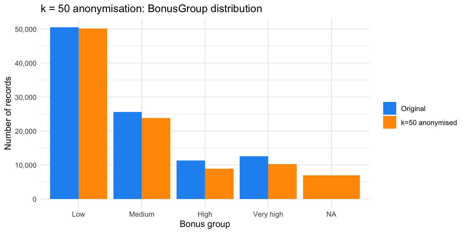
Reading this: global risk falls 0.77% → 0.41% (about 47%). All suppression lands on BonusGroup (6.9%) and ValueGroup (0.44%) — importance always spends the cheapest variable first.

Note

Effective for small datasets or fine-grained geography. For large datasets, suppression rates are low at small k but rise quickly as k grows, as shown above. k-anonymity also cannot handle continuous variables well, and does not protect sensitive values (the claims column is untouched).

This is the case study’s reinsurer question in miniature: even at k=50, ValueGroup and BonusGroup are the only things touched — Gender, AgeGroup, and DensityGroup, the variables a reinsurer with partial background knowledge would most likely already know, are completely untouched by this suppression. That’s exactly why k-anonymity alone is a weak answer for that specific recipient.

💬 Discuss (3 min)

k-anonymity doesn’t protect the sensitive column, only the ability to link a record to a person.

Is that real privacy protection, or false comfort?

A way to think about it: both, depending on what’s in the sensitive column. It closes the linkage channel, real protection, but says nothing about attribute inference within a suppressed group (if everyone in a group of 50 filed the same type of claim, k-anonymity doesn’t hide that). This exact gap is why extensions like l-diversity (Chapter 6) exist.

Break — 10 min

Part 4 — Differential privacy

The Laplace mechanism

Adds calibrated noise to a statistic before release (Dwork et al. 2006):

\mathcal{M}(D) = f(D) + \text{Lap}\!\left(\frac{\Delta f}{\varepsilon}\right)

Smaller \varepsilon → more noise → stronger privacy, less utility.

Δf is the sensitivity: the most a single record could change the statistic if it were added or removed, a different sense of “sensitive” from the claims column discussed earlier in this deck. Lap() draws random noise from a Laplace distribution, a symmetric, bell-like curve centred on zero. For a mean over n bounded values, sensitivity = (upper-lower)/n — this single fact is the whole story of the next two slides.

Noise depends on group size, not just \varepsilon

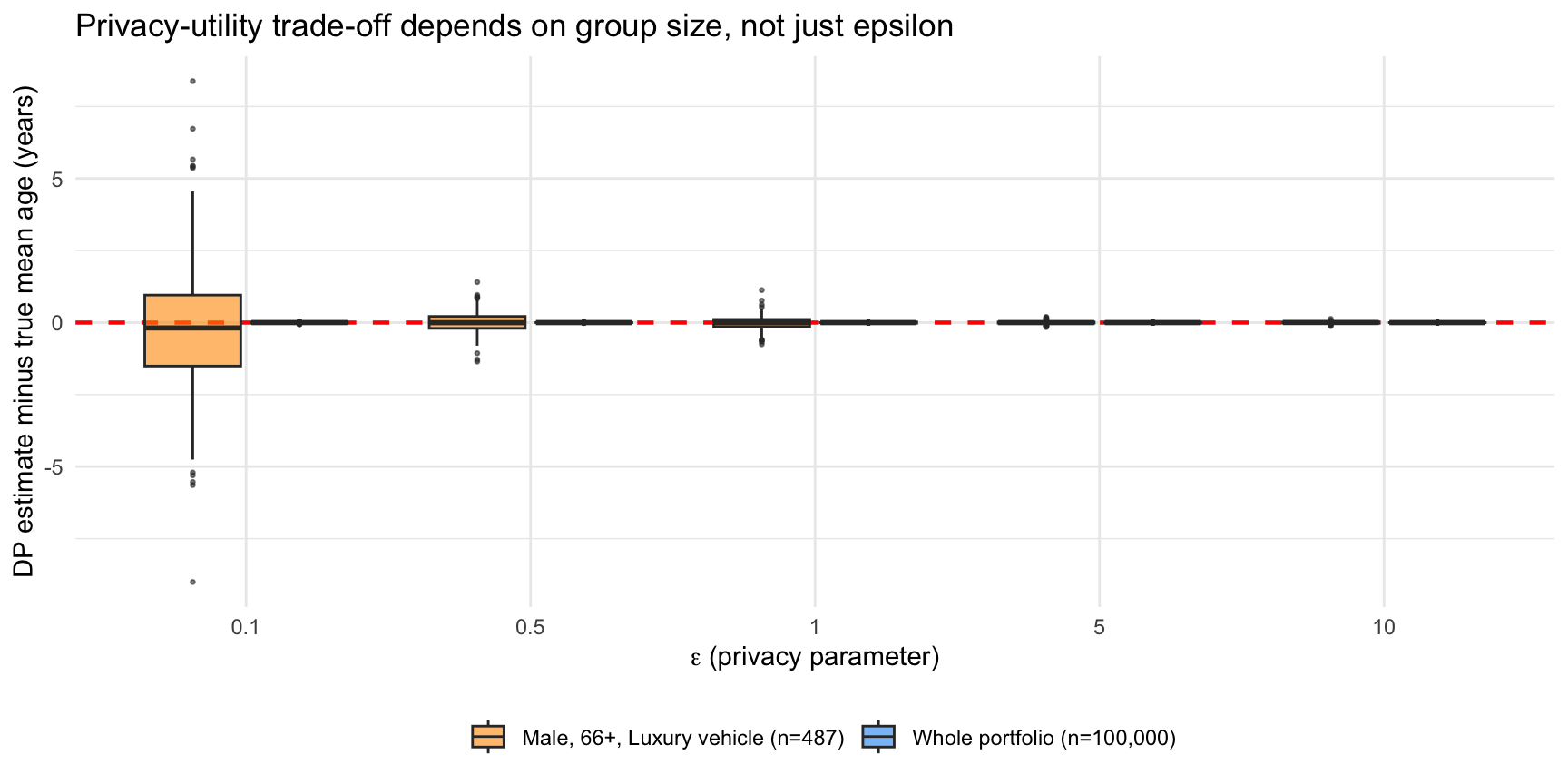
Reading this: whole portfolio (n=100,000) noise is invisibly small at every \varepsilon. The same mechanism, same \varepsilon, on the n=487 rare subgroup from Part 2, swings multiple years at \varepsilon=0.1.

Sensitivity scales as 1/n. A portfolio-wide statistic is nearly free to protect with DP; a fine-grained breakdown is not.

With n = 100,000, sensitivity of mean age ≈ 0.0008 — even ε = 0.1 gives usably small noise, which is why a static table of DP estimates for the whole portfolio looks unchanged across every epsilon value: it isn’t a mistake, it’s what large n predicts. The n=487 group is the same “Male, 66+, Luxury vehicle” combination introduced in the aggregation-problem slide in Part 2. This is also why the 2018 US Census reconstruction attack, discussed in Chapter 6, was hardest to defend against at the smallest published geographies (census blocks), not at state or national level — small n, large sensitivity, more noise needed for the same guarantee.

Interpreting epsilon

ε	Whole portfolio (n=100,000)	Rare subgroup (n=487)	Interpretation
0.1	Negligible	Very large (multi-year)	Strong privacy; fine for portfolio stats, unusable for small groups
0.5–1	Negligible	Large–moderate	Common default for aggregates
5	Negligible	Small	Acceptable even for moderately small groups
10	Negligible	Very small	Weak privacy, close to raw output

Composition matters: k independent queries at ε each consume a total budget of kε (basic composition). This table is also the direct evidence for the case study’s vendor question — a vendor asking for one or two portfolio-wide statistics can be served at a strict epsilon almost for free, but if a regulator later asks for the same breakdown by a small subgroup (say, by postcode), the vendor’s request moves into the right-hand column of this table, and the same epsilon is no longer free.

💬 Discuss (4 min)

Setting epsilon for your organisation’s next public data release.

ε = 0.5 (strong privacy, noisy) or ε = 5 (weaker privacy, useful)? What decides it?

A way to think about it: it depends on n more than on any fixed rule. For a portfolio-wide statistic like this chapter’s examples, \varepsilon=0.5 already costs almost nothing, so there’s little reason to accept the weaker guarantee of \varepsilon=5. The trade-off only starts to bite once the statistic is computed over a small group.

Part 5 — Synthetic data

Desired properties of synthetic data

Synthetic data generators are judged on three properties, which do not automatically move together (Jordon et al. 2022):

• Fidelity — does the synthetic distribution resemble the real one, marginally and jointly?
• Utility — does it actually support the downstream task, not just look similar?
• Privacy — does releasing it leak information about specific real individuals?

A generator that memorised the training data scores perfectly on fidelity and utility, and fails privacy completely. The checks that follow test all three, in that order.

This framework is why the fidelity checks (marginals, coefficients) are not the end of the evaluation — a synthetic dataset can look statistically similar and still be useless for its actual purpose, or still leak individuals. The order matters pedagogically too: a dataset that fails fidelity isn’t worth testing further for utility or privacy.

Generating with synthpop

Fits a sequence of conditional models, one variable at a time (CART by default), sampling new synthetic records from the fitted sequence, not resampling real ones.

CART stands for Classification and Regression Trees, a method that predicts each variable by repeatedly splitting the data into groups based on the other variables. Critically, CART draws each synthetic value from the actual observed values in the matching leaf node, not a smoothed or interpolated value — this single fact explains both the good fidelity results and the NNDR spike a few slides from now. A 2,000-record real holdout is set aside before synthesis, kept aside purely to test generalisation later.

Fidelity: marginal distributions

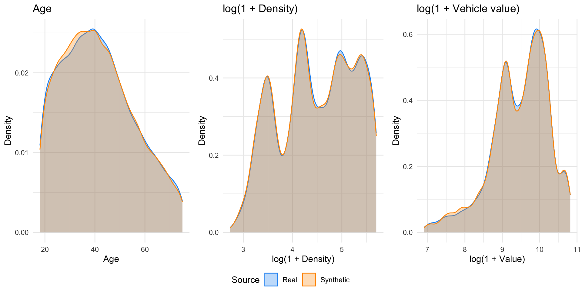
Synthetic distributions closely track the real ones for Age, Density, and Value.

Density and Value are plotted as log(1+x), not raw, because both are heavily right-skewed (a long tail of dense-urban locations and luxury vehicles) — a raw-scale plot would compress almost every record into a spike near zero and hide any real fidelity gap inside it. log1p rather than plain log stays defined at x=0, which matters since some records have Density or Value near zero.

Evaluating utility: TSTR

Train-synthetic-test-real: fit a model on synthetic data, evaluate it on real records synthesis never saw. This tests the thing a downstream user actually does with the data, not just resemblance.

Model trained on	AUC on 2,000-record real holdout
Real data	0.728
Synthetic data	0.729

A negligible, even reversed, gap. A model built entirely on synthetic data performs just as well on real future business as one built on the real data it was meant to protect.

This directly answers the reinsurer’s question from the case study: they wanted assurance that a pricing model built on synthetic data would actually work on real future business. The AUC gap here (0.001) is the strongest evidence in the whole chapter that synthetic data can substitute for real record-level data for that specific purpose. Coefficient agreement (checked earlier) is a weaker, resemblance-only test by comparison — TSTR is the direct one.

Evaluating privacy: NNDR

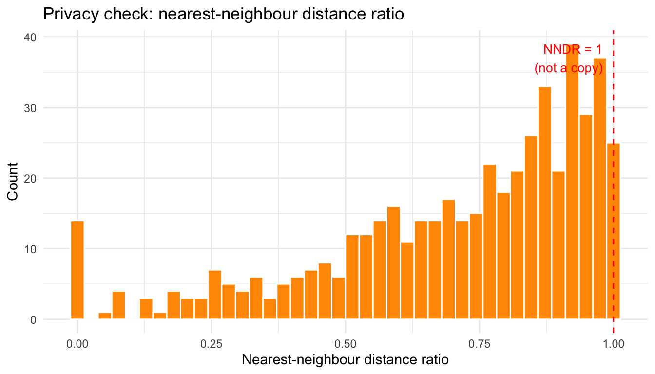
\text{NNDR} = \frac{d(\text{syn}_i, \text{real nearest})}{d(\text{syn}_i, \text{real 2nd nearest})}

Near 1 = not a copy. Near 0 = memorisation risk.

There is a real spike near 0: ~4% of sampled records (20 of 500) exactly match a real record on Age/Density/Value. Not memorisation — Density has only 471 distinct values in 8,000 records, so CART’s leaf-resampling can coincidentally reproduce one real combination. The categorical columns (Group1, Bonus) still typically differ.

Important

NNDR on numeric columns is only one test. A complete evaluation also checks membership inference (can an attacker tell whether a specific record was used to train the model?) and attribute inference (can an attacker guess a sensitive field about someone from the synthetic data?) (Jordon et al. 2022).

This is exactly the “generates each value from actual observed data” property flagged on the synthpop slide earlier. The spike is a genuine, explainable finding, not a bug and not something to round down to “no risk” — it’s precisely the kind of residual risk membership-inference testing exists to catch, and it’s why the case study’s answer for the reinsurer flags this as a caveat rather than an all-clear.

💬 Discuss (4 min)

NNDR near 1 says most synthetic records aren’t copies of real ones — but a small share are exact matches on the numeric columns checked.

Does that change whether the dataset is safe to release? What else would you want to check?

A way to think about it: not an automatic block, but not an all-clear either. A 4% exact-match rate on the checked variables means membership-inference testing should happen before release, not that release should be blocked outright — the same “additional testing needed” conclusion the callout below reaches.

Wrap-up

Controls by lifecycle stage

Stage	Key controls
Collection	Minimum necessary, document legal basis
Storage	Pseudonymise, encrypt, role-based access
Analytics	Purpose limitation, k-anonymise/DP before analyst access
Output/sharing	Aggregate only, DP noise, data-sharing agreements
Retention	Automated deletion, secure disposal

Case study, resolved: answering the three questions

1. Which recipient could get k-anonymised data? Arguably none — wrong tool for all three requests, not a flaw in k-anonymity itself. Where it would otherwise apply, the reinsurer’s background knowledge weakens it further: this chapter’s own k=50 result left Gender/AgeGroup/DensityGroup untouched, exactly what a repeat treaty partner might already know.
2. Does the pricing team need synthetic data? No — the simpler answer is governance only: purpose limitation and role-based access. They’re internal, already trusted, and validated against live production regardless of training data.
3. Does the vendor’s aggregate-only need rule out two techniques? Yes. k-anonymity and synthetic data both protect files; the vendor never receives one. Differential privacy is the only relevant technique of the three.

In short: reinsurer → synthetic data (TSTR: AUC 0.728 vs 0.729). Internal team → governance alone. Vendor → differential privacy. Three recipients, three different tools.

This is the payoff of opening with the case study: by the end of the chapter, “which PET should we use” has become “it depends on the recipient, and here is how you’d show your working” — exactly the muscle Chapter 8’s trade-offs discussion will ask students to use again across fairness, explainability, and privacy together.

💬 Discuss (5 min) — wrap-up

Looking at the lifecycle-controls table, and the case study resolution above.

Which stage — or which recipient-matching decision — does an organisation you know handle worst?

Summary

• Re-identification risk is real even in large “anonymised” datasets
• k-anonymity: reduces identifiability, doesn’t protect sensitive values, loses utility once k is large enough to matter
• Differential privacy: mathematical guarantee, scales well with n — the same \varepsilon costs far more for a small subgroup than a large portfolio
• Synthetic data (synthpop/CART): evaluated on fidelity, utility (TSTR), and privacy (NNDR) — good on all three here, with a genuine, explainable minority-match caveat
• No single technique is sufficient alone, and no single technique fits every recipient — layered, recipient-matched controls are required

Recommended reading

• Templ (2017); Sweeney (2002) — sdcMicro and k-anonymity
• Dwork et al. (2006) — original ε-DP paper
• Nowok et al. (2016); Jordon et al. (2022) — synthetic data generation and evaluation

Next class

Chapter 8 — Trade-offs, Integration, and Governance

Bring one open question from Chapters 1–7 you’d like the course to tie together.

Dwork, Cynthia, Frank McSherry, Kobbi Nissim, and Adam Smith. 2006. “Calibrating Noise to Sensitivity in Private Data Analysis.” Theory of Cryptography, 265–84.

Franconi, Luisa, and Silvia Polettini. 2004. “Individual Risk Estimation in \mu-Argus: A Review.” In Privacy in Statistical Databases, vol. 3050. Lecture Notes in Computer Science. Springer.

Jordon, James, Lukasz Szpruch, Florimond Houssiau, et al. 2022. “Synthetic Data – What, Why and How?” arXiv Preprint arXiv:2205.03257.

Nowok, Beata, Gillian M Raab, and Chris Dibben. 2016. “Synthpop: Bespoke Creation of Synthetic Data in r.” Journal of Statistical Software 74 (11): 1–26.

Sweeney, Latanya. 2002. “K-Anonymity: A Model for Protecting Privacy.” International Journal of Uncertainty, Fuzziness and Knowledge-Based Systems 10 (5): 557–70.

Templ, Matthias. 2017. Statistical Disclosure Control for Microdata: Methods and Applications in r. Springer.