---
title: "Fairness Practice"
urlcolor: blue
bibliography: reference.bib
resources:
- data/pg15training_processed.csv
other-links:
- text: In-class slides
href: Slides-Fairness-Practice.slides.html
icon: easel2
format:
html:
code-tools: true
code-fold: true
format-links: false
pdf:
documentclass: article
pdf-engine: xelatex
toc: true
toc-depth: 3
geometry: margin=0.6in
fontsize: 9pt
colorlinks: true
include-in-header:
text: |
\usepackage{fvextra}
\fvset{breaklines,breakanywhere}
execute:
echo: true
warning: false
message: false
---
## Learning objectives
- Operationalise a chosen fairness criterion end-to-end: pick an intervention stage, implement it, and measure both fairness and accuracy.
- Implement the MU, MDP, MCDP, and MC model designs from Chapter 2 (GLM and XGBoost) on a worked case study.
- Measure the fairness–accuracy trade-off using the disparate impact ratio and RMSE.
- Interpret outcome redistribution across protected and legitimate subgroups.
- Apply the same M0/MU framework to a binary classification problem, using standard classification-fairness metrics (demographic parity, equalized odds, predictive rate parity).
- Apply a post-processing correction (`roc_pivot`) to a classifier, and observe the trade-off it creates across criteria, not just against accuracy.
## From principle to practice
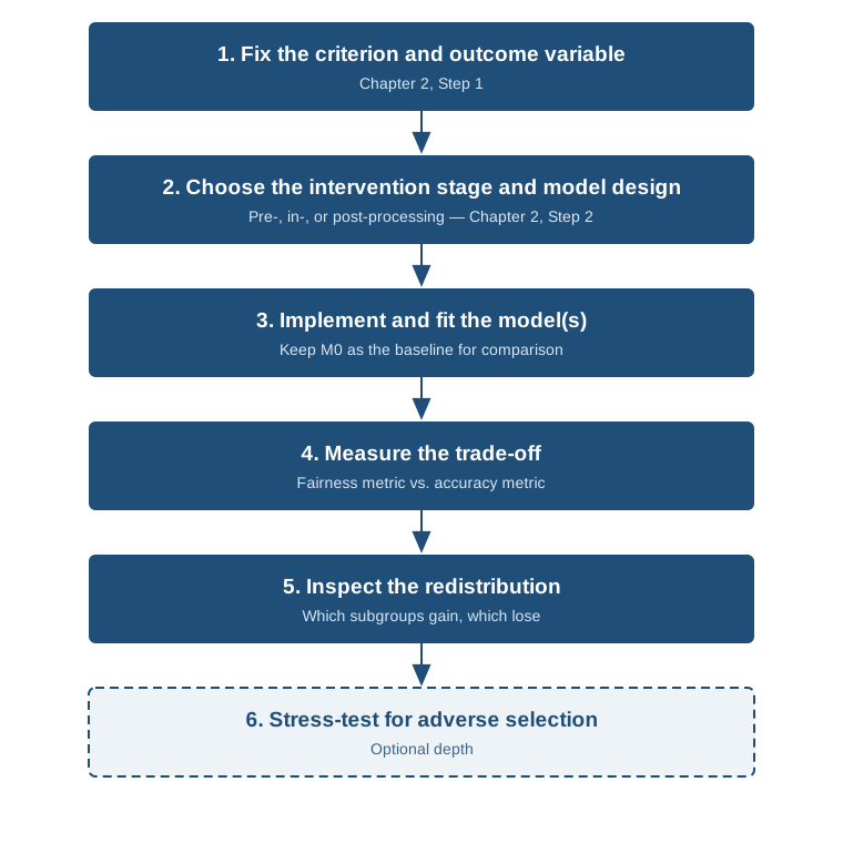
Chapter 2 introduced *what* fairness criterion to choose and *which* model design (M0, MU, MDP, MCDP, MC) enforces it. Turning that choice into a working system follows the same sequence regardless of domain:
1. **Fix the criterion and the outcome variable** the criterion applies to (Chapter 2, Step 1).
2. **Choose the intervention stage** (pre-, in-, or post-processing) and the corresponding model design (Chapter 2, Step 2).
3. **Implement and fit** the model(s), keeping a baseline (M0) for comparison.
4. **Measure the trade-off**: a fairness metric (e.g. disparate impact ratio) against an accuracy metric (e.g. RMSE), not in isolation.
5. **Inspect the redistribution**: which subgroups gain and which lose relative to the current benchmark.
6. **Stress-test for adverse selection** (optional depth): check whether the fairer model systematically disagrees with the benchmark on a segment where actual outcomes favour one model over the other. See [fair.feihuang.org's Case Study: Fair Models](https://fair.feihuang.org/Case%20Study%202/case_study2.html) for a worked double-lift-chart analysis of this step.
{fig-align="center" width="80%"}
This lecture works through steps 3–5 in full, on a single worked case study, so each step above has a concrete implementation to point to.
## Case study: fair pricing for motor insurance
Consider a mid-sized French motor insurer whose Chief Actuary must sign off on a new pricing model before it reaches production. Regulators in several markets, from Colorado's SB21-169 to the EU's unisex-pricing rule, now require insurers to show that a pricing model does not unfairly disadvantage a protected group before deployment. Getting this wrong is costly either way. An unfair model risks fines, litigation, and reputational damage, while an overcorrected model can misprice risk and erode profitability. The Chief Actuary needs a defensible way to compare model designs on both fairness and accuracy before choosing one.
We use [Case Study: Fair Models](https://fair.feihuang.org/Case%20Study%202/case_study2.html) from the Fair Pricing Playbook [@huang2026fairpricingplaybook], based on the model designs and empirical results in @xin2024antidiscrimination, as the worked example. The workflow above (fix criterion → choose stage → fit → measure trade-off → inspect redistribution → stress-test) applies equally to a hiring, lending, or healthcare-allocation model.
We use French motor insurance data to compare five pricing models, ranging from a full baseline to four anti-discrimination designs, using both GLMs and XGBoost.
::: {.callout-tip}
Read Chapter 2 (Fairness Principles) first. The five model designs implemented here each correspond to a fairness criterion introduced in Chapter 2.
:::
# Setup
## Data: French motor insurance
We use the `pg15training` dataset. A processed CSV ([`data/pg15training_processed.csv`](data/pg15training_processed.csv)) is provided alongside this chapter, with `InsuranceScore` and the other model predictors already built from the raw policy data, so reproducing the code below does not require installing `CASdatasets` [@dutang2020package] or reconstructing these variables.
- 100,021 third-party liability (TPL) motor policies, 2009–2010 (third-party liability covers injury or damage the policyholder causes to others, not their own vehicle)
- Response: **pure premium** = claim frequency (how often a policyholder makes a claim) × claim severity (the average cost per claim). Pure premium is roughly the expected claims cost per policy, before any margin is added.
- Protected attribute: **Gender**
- Legitimate rating variables: Age, Bonus (a no-claims discount level, sometimes called bonus-malus, where lower means fewer past claims), GroupOne (vehicle group), Density, Value
- Non-legitimate variable: **InsuranceScore** (acts as a credit-score proxy, constructed from type, category, occupation, region, and age via logistic regression)
The first 21 duplicate records are removed. Final sample: 100,021 - 21 = 100,000 policies.
## Why InsuranceScore as the non-legitimate variable?
The baseline scenario in @xin2024antidiscrimination treats `InsuranceScore` as the sole non-legitimate variable. It stands in for a proxy-rich factor (like a credit-based insurance score) that:
- Retains some predictive value for claim risk
- May correlate with the protected attribute (gender)
- Attracts stricter fairness scrutiny in some regulatory regimes
This construction also serves a practical purpose. The disparate-impact remover requires continuous inputs, so summarising categorical proxies into one score makes debiasing feasible under MCDP.
## The five models
| Model | Paper notation | Description |
|-------|---------------|-------------|
| Model 1 | M0 | Full model, includes Gender |
| Model 2 | MU | Unawareness, Gender removed |
| Model 3 | MDP | All predictors debiased before training |
| Model 4 | MCDP | Only InsuranceScore debiased, legitimate variables unchanged |
| Model 5 | MC | Full model fitted, predictions averaged over gender at scoring |
Each model is fitted with both **GLM** (Poisson frequency + Gamma severity) and **XGBoost**.
```{r packages}
#| code-fold: true
#| code-summary: "Package setup"
library(fairmodels)  # disparate_impact_remover() and roc_pivot(), the pre- and post-processing corrections used below
library(tidyverse)   # data wrangling (dplyr) and plotting (ggplot2) throughout
library(ggpubr)      # ggarrange(), combining fairness-accuracy and redistribution plots into single figures
library(scales)      # scales::percent, formatting axis labels as percentages
library(knitr)       # kable(), rendering summary tables
library(kableExtra)  # kable_styling(), formatting kable() tables for HTML/PDF output
library(xgboost)     # xgb.train() and xgb.DMatrix(), the XGBoost model class fitted alongside GLM

set.seed(14)     # fixes R's random-number generator so the jittering used in the disparate-impact remover below is reproducible
lambda_all <- 1  # strength of the disparate-impact remover's debiasing (0 = no correction, 1 = full correction); used for both MDP and MCDP below
```
## Loading and preparing the data
```{r}
#| code-fold: true
#| code-summary: "Load the processed data"
# read.csv() loads the data; the %>% pipe passes it into mutate(), which adds/
# changes columns without a separate assignment step for each one.
ClaimsData <- read.csv("data/pg15training_processed.csv", stringsAsFactors = FALSE) %>%
  mutate(
    Gender   = relevel(as.factor(Gender), ref = "Male"),  # treat Gender as categorical; relevel() sets "Male" as the reference level, so model coefficients are read as "relative to Male"
    Female   = as.integer(Gender == "Female"),             # a 0/1 numeric version of Gender, needed later for the MC averaging step
    Age      = as.factor(as.integer(Age)),                 # categorical version of Age, used by the GLMs below (the continuous version, Age.ct, already exists in the CSV)
    Bonus    = as.factor(as.integer(Bonus)),
    GroupOne = as.factor(as.integer(GroupOne))
  )

# Claim severity (cost per claim) can only be modelled on policies that actually
# had a claim, so we keep a second data frame filtered to Indtppd > 0 (positive claims).
ClaimsData_rd <- ClaimsData %>% filter(Indtppd > 0)
```
# Pre-processing
## Debiasing with the disparate-impact remover
For MDP (Model 3) and MCDP (Model 4), we pre-process predictors using the **disparate-impact remover** [@feldman2015certifying], implemented in the `fairmodels` R package.
The remover adjusts continuous variable distributions so that they no longer depend on the protected attribute (gender), while preserving the overall distribution shape.
- **MDP**: apply to all selected predictors (Age, Bonus, Value, Density, GroupOne, InsuranceScore)
- **MCDP**: apply only to the non-legitimate variable (InsuranceScore)
A small amount of random noise is added to ordinal variables before debiasing to avoid tied-value problems. After debiasing, ordinal variables are mapped back to their original factor levels.
```{r}
#| code-fold: true
#| code-summary: "Show scenario and helper function definitions"
# InsuranceScore is the one predictor treated as "non-legitimate" (a proxy variable);
# everything else in glm_predictors is treated as legitimate. This split is what
# distinguishes MDP (debias everything) from MCDP (debias only non_legitimate).
non_legitimate <- c("Insurancescore")

glm_predictors <- c("Age.ct", "Bonus", "Value", "Density", "GroupOne", "Insurancescore")
xgb_predictors <- glm_predictors

# Turns continuous Age (in years) into age-band labels like "18-22", "23-27", ...
# Needed because the debiasing step below works on continuous variables, but the
# GLMs use Age as a categorical (banded) predictor, so we have to re-band it afterwards.
make_age_group <- function(age) {
  cut(age,
    breaks = c(-Inf, 22, 27, 32, 37, 42, 47, 52, 57, 62, 67, Inf),
    labels = c("18-22","23-27","28-32","33-37","38-42","43-47","48-52","53-57","58-62","63-67","68+"),
    right = TRUE)
}

# Rounds a continuous (debiased) variable back to its nearest original integer level,
# clipped to [min_level, max_level]. Used to turn Bonus and GroupOne back into the
# same discrete categories they started as, after the debiasing step treats them as continuous.
bin_to_factor <- function(x, min_level, max_level) {
  levels <- min_level:max_level
  x <- pmin(pmax(x, min_level), max_level)        # clip: nothing below min_level or above max_level
  cuts <- c(min_level - 0.5, levels[-1] - 0.5, max_level + 0.5)
  as.factor(as.numeric(cut(x, breaks = cuts, labels = levels, include.lowest = TRUE)))
}

# Builds a debiased copy of `data`: runs disparate_impact_remover() on the columns
# named in features_to_transform (all predictors for MDP, or just InsuranceScore for MCDP),
# so their distributions no longer depend on Gender.
make_di_removed_data <- function(data, features_to_transform, lambda = 1) {
  data_for_di <- data %>%
    # disparate_impact_remover() needs continuous inputs, so Bonus and GroupOne
    # (currently categorical) are temporarily converted to numeric here.
    mutate(GroupOne.ct = as.numeric(GroupOne), Bonus.ct = as.numeric(Bonus))

  # Adds tiny random noise (jitter) to break ties between repeated values, which the
  # debiasing algorithm needs to rank-order observations. The smallest and largest
  # values of each variable are left untouched (`keep`) so the range doesn't change.
  jitter_keep_minmax <- function(x, factor = 1) {
    keep <- x == min(x, na.rm=TRUE) | x == max(x, na.rm=TRUE)
    x[!keep] <- jitter(x[!keep], factor = factor)
    x
  }

  # Apply jitter_keep_minmax() to every variable that will be debiased below.
  # GroupOne.ct gets a larger factor (5) because it is a coarse integer code with many
  # more tied values than the other variables, so it needs more noise to break the ties.
  data_for_di <- data_for_di %>%
    mutate(
      Age.ct = jitter_keep_minmax(Age.ct, factor=1),
      Bonus.ct = jitter_keep_minmax(Bonus.ct, factor=1),
      Value = jitter_keep_minmax(Value, factor=1),
      Density = jitter_keep_minmax(Density, factor=1),
      GroupOne.ct = jitter_keep_minmax(GroupOne.ct, factor=5),
      Insurancescore = jitter_keep_minmax(Insurancescore, factor=1)
    )

  # The actual debiasing step: adjusts each column in features_to_transform so its
  # distribution is the same for every Gender group. `lambda = 1` applies the full
  # correction (lambda = 0 would leave the data unchanged).
  di_data <- disparate_impact_remover(
    data = data_for_di, protected = as.factor(data_for_di$Gender),
    features_to_transform = features_to_transform, lambda = lambda
  )

  # Convert Age, GroupOne, and Bonus back from continuous (post-debiasing) values
  # to the categorical bands the GLMs expect, using the two helpers defined above.
  di_data <- di_data %>%
    mutate(
      Age = make_age_group(Age.ct),
      Age = as.factor(as.numeric(Age)),
      GroupOne = bin_to_factor(GroupOne.ct, 1, 20),
      Bonus = bin_to_factor(Bonus.ct, 1, 21)
    )
  di_data
}

# Thin wrappers around glm() that fix the distribution family for each part of the
# frequency-severity model: Gamma for claim severity (cost, always positive, right-skewed),
# Poisson for claim frequency (a count). Wrapping them avoids repeating the family=...
# argument on every one of the eight glm() calls used across the four model designs below.
fit_gamma_model  <- function(formula, data) glm(formula, family=Gamma(link="log"), data=data)
fit_poisson_model <- function(formula, data) glm(formula, family=poisson(link="log"), data=data, offset=log(Exppdays))

# Rescales a vector of raw predicted premiums so its total matches a reference
# portfolio's total (used later so every model's overall book size is comparable,
# and only the *distribution* of premiums across policyholders differs).
adjust_to_base_portfolio <- function(raw_premium, base_premium) raw_premium * sum(base_premium) / sum(raw_premium)

# XGBoost needs a numeric matrix, not a data frame of factors, so this turns every
# categorical predictor into 0/1 dummy columns (model.matrix()) and drops the columns
# XGBoost doesn't use (e.g. the outcome variables, or the redundant reference level GenderMale).
make_xgb_design <- function(data) {
  # Each entry is dropped for a different reason, not because XGBoost can't handle it:
  # - "Age": the banded/categorical version of age. The model uses the continuous
  #   Age.ct instead (kept), so Age would just duplicate the same information.
  # - "GroupOne.ct" and "Bonus.ct": continuous numeric versions of GroupOne and Bonus,
  #   left over from the disparate-impact remover's internal calculations (present only
  #   in the debiased data, ClaimsData_DIremv). The model uses the categorical GroupOne
  #   and Bonus (kept) as the actual rating factors, so these would duplicate them.
  # - "Female": a 0/1 duplicate of Gender, needed only for the MC gender-averaging step
  #   elsewhere; model.matrix() below already one-hot-encodes Gender itself.
  # - "ClaimSeverity": the outcome variable for the GLM severity model. XGBoost's
  #   severity target is Indtppd instead, so ClaimSeverity must never appear as a
  #   predictor or it would leak the answer into the model.
  xgb_unused <- c("Age","GroupOne.ct","Bonus.ct","Female","ClaimSeverity")
  data %>%
    select(-any_of(xgb_unused)) %>%
    model.matrix(~ 0 + ., data=.) %>%
    as.data.frame() %>%
    select(-any_of("GenderMale"))
}

# Packages a predictor matrix into the xgb.DMatrix format XGBoost's training/prediction
# functions require. `base_margin` supplies a known offset on the log scale (e.g. exposure
# for frequency, or the fitted frequency for severity) so XGBoost only has to learn the
# remaining pattern, not the offset itself. `response` is omitted when just predicting.
make_xgb_dmatrix <- function(data, response=NULL, base_margin, drop_vars) {
  x <- data %>% select(-any_of(drop_vars)) %>% as.matrix()
  if (is.null(response)) dmat <- xgb.DMatrix(x)
  else dmat <- xgb.DMatrix(x, label=data[[response]])
  setinfo(dmat, "base_margin", log(base_margin))
  dmat
}

# Ensures a new dataset has exactly the same dummy-variable columns, in the same order,
# as the data XGBoost was trained on (any column missing in new_data is filled with 0).
# Needed because model.matrix() can produce slightly different columns for training vs.
# scoring data if a category happens to be absent from one of the two.
align_xgb_design <- function(new_data, train_data) {
  missing_cols <- setdiff(names(train_data), names(new_data))
  if (length(missing_cols) > 0) new_data[missing_cols] <- 0
  new_data[, names(train_data), drop=FALSE]
}
```
```{r}
#| code-fold: true
#| code-summary: "Build debiased datasets"
# Debias ALL predictors (Age, Bonus, Value, Density, GroupOne, InsuranceScore) once;
# Model 3 (MDP) and Model 4 (MCDP) below each take only the columns they need from this.
features_to_transform <- c("Age.ct","Bonus.ct","Value","Density","GroupOne.ct","Insurancescore")
ClaimsData_DIremv <- make_di_removed_data(ClaimsData, features_to_transform, lambda=lambda_all)

# Model 3 = MDP: replace every legitimate + non-legitimate predictor with its debiased version.
ClaimsData_M3 <- ClaimsData
ClaimsData_M3[, c("Age","Age.ct","Bonus","Value","Density","GroupOne","Insurancescore")] <-
  ClaimsData_DIremv[, c("Age","Age.ct","Bonus","Value","Density","GroupOne","Insurancescore")]

# Model 4 = MCDP: replace ONLY the non-legitimate predictor (InsuranceScore) with its
# debiased version; every legitimate predictor keeps its original, undebiased values.
ClaimsData_M4 <- ClaimsData
m4_features <- intersect(glm_predictors, non_legitimate)
ClaimsData_M4[, m4_features] <- ClaimsData_DIremv[, m4_features]

# Claims-only versions, needed for fitting the severity (Gamma) models.
ClaimsData_M3_rd <- ClaimsData_M3 %>% filter(Indtppd > 0)
ClaimsData_M4_rd <- ClaimsData_M4 %>% filter(Indtppd > 0)
```
# Fitting the models
## GLM frequency–severity framework
Both GLM and XGBoost use a **frequency–severity** decomposition:
$$\text{Pure Premium} = \text{Claim Frequency} \times \text{Claim Severity}$$
- **Frequency**: Poisson GLM with log link and exposure offset (exposure is how long, in days, the policy was active and at risk of a claim)
- **Severity**: Gamma GLM with log link (fitted on claims-only data)
Age is entered as a continuous function ($\text{Age}, \log(\text{Age}), \text{Age}^2, \text{Age}^3, \text{Age}^4$) following @schelldorfer2019nesting.
```{r}
#| code-fold: true
#| code-summary: "Fit GLM models"
# sev_formula_m1 is the severity formula WITH Gender (used for M0); update(..., . ~ . - Gender)
# removes Gender from an existing formula rather than retyping it, giving sev_formula_m2
# (used for MU, MDP, MCDP, which all exclude Gender as a direct predictor).
sev_formula_m1 <- ClaimSeverity ~ Age.ct + log(Age.ct) + I(Age.ct^2) + I(Age.ct^3) +
  I(Age.ct^4) + Bonus + Density + Gender + Insurancescore
sev_formula_m2 <- update(sev_formula_m1, . ~ . - Gender)

# Same idea for the frequency formula. Note GroupOne (vehicle group) appears here but
# not in the severity formula, since it is a rating factor used for frequency only.
freq_formula_m1 <- Numtppd ~ Age.ct + log(Age.ct) + I(Age.ct^2) + I(Age.ct^3) +
  I(Age.ct^4) + Bonus + Density + GroupOne + Insurancescore + Gender
freq_formula_m2 <- update(freq_formula_m1, . ~ . - Gender)

# Severity (Gamma) models: 1 = M0 (with Gender), 2 = MU (Gender removed, original data),
# 3 = MDP (Gender removed, all predictors debiased), 4 = MCDP (Gender removed, only
# InsuranceScore debiased). Same formula, different input data, is what tells the four
# model designs apart.
SevGamma1  <- fit_gamma_model(sev_formula_m1, ClaimsData_rd)
SevGamma2  <- fit_gamma_model(sev_formula_m2, ClaimsData_rd)
SevGamma3  <- fit_gamma_model(sev_formula_m2, ClaimsData_M3_rd)
SevGamma4  <- fit_gamma_model(sev_formula_m2, ClaimsData_M4_rd)

# Frequency (Poisson) models, same four-design pattern as above.
FreqPoisson1 <- fit_poisson_model(freq_formula_m1, ClaimsData)
FreqPoisson2 <- fit_poisson_model(freq_formula_m2, ClaimsData)
FreqPoisson3 <- fit_poisson_model(freq_formula_m2, ClaimsData_M3)
FreqPoisson4 <- fit_poisson_model(freq_formula_m2, ClaimsData_M4)
```
```{r}
#| code-fold: true
#| code-summary: "Fit XGBoost models"
# Build the numeric design matrices XGBoost needs, one for the original data and one
# for the fully-debiased (MDP) data, then splice the debiased InsuranceScore column into
# a copy of the original design to get the MCDP design (mirrors the GLM logic above).
xgbData    <- make_xgb_design(ClaimsData)
xgbData_M3 <- make_xgb_design(ClaimsData_DIremv)
xgbData_M4 <- xgbData
m4_train_vars <- intersect(names(xgbData_M4), non_legitimate)
xgbData_M4[, m4_train_vars] <- xgbData_M3[, m4_train_vars]

# Columns every frequency/severity DMatrix must drop: the outcome variables themselves
# (Numtppd, Indtppd) and the exposure column (Exppdays, used separately as the offset).
drop_common <- c("Exppdays","Numtppd","Indtppd")

# One DMatrix per model design for claim FREQUENCY (the count target Numtppd).
# FM1 keeps Gender (M0); FM2/FM3/FM4 drop GenderFemale (MU/MDP/MCDP) and differ only
# in which underlying data (original vs. debiased) they were built from.
xgbData_FM1 <- make_xgb_dmatrix(xgbData, "Numtppd", xgbData$Exppdays, drop_common)
xgbData_FM2 <- make_xgb_dmatrix(xgbData, "Numtppd", xgbData$Exppdays, c(drop_common,"GenderFemale"))
xgbData_FM3 <- make_xgb_dmatrix(xgbData_M3,"Numtppd",xgbData_M3$Exppdays,c(drop_common,"GenderFemale"))
xgbData_FM4 <- make_xgb_dmatrix(xgbData_M4,"Numtppd",xgbData_M4$Exppdays,c(drop_common,"GenderFemale"))

# XGBoost hyperparameters for the frequency models. count:poisson mirrors the Poisson
# GLM's distributional assumption for a claim count; max_depth/eta/subsample control
# how complex and how slowly-learning each tree ensemble is (kept shallow to avoid overfitting).
paramsFreq <- list(objective="count:poisson", eval_metric="poisson-nloglik",
  max_depth=2, eta=0.05, min_child_weight=3, subsample=0.8, colsample_bytree=0.8, tree_method="hist")

set.seed(358)  # fixes XGBoost's internal randomness (row/column subsampling) so results are reproducible
xgbFreq1 <- xgb.train(xgbData_FM1, nrounds=3958, params=paramsFreq)
xgbFreq2 <- xgb.train(xgbData_FM2, nrounds=3988, params=paramsFreq)
xgbFreq3 <- xgb.train(xgbData_FM3, nrounds=3151, params=paramsFreq)
xgbFreq4 <- xgb.train(xgbData_FM4, nrounds=3987, params=paramsFreq)

# Same idea for claim SEVERITY (cost per claim), fitted on claims-only rows (Indtppd > 0).
xgbData_sev    <- xgbData    %>% filter(Indtppd > 0)
xgbData_M3_sev <- xgbData_M3 %>% filter(Indtppd > 0)
xgbData_M4_sev <- xgbData_M4 %>% filter(Indtppd > 0)

xgbData_SM1 <- make_xgb_dmatrix(xgbData_sev,   "Indtppd", xgbData_sev$Numtppd,   drop_common)
xgbData_SM2 <- make_xgb_dmatrix(xgbData_sev,   "Indtppd", xgbData_sev$Numtppd,   c(drop_common,"GenderFemale"))
xgbData_SM3 <- make_xgb_dmatrix(xgbData_M3_sev,"Indtppd", xgbData_M3_sev$Numtppd,c(drop_common,"GenderFemale"))
xgbData_SM4 <- make_xgb_dmatrix(xgbData_M4_sev,"Indtppd", xgbData_M4_sev$Numtppd,c(drop_common,"GenderFemale"))

# reg:gamma mirrors the Gamma GLM's distributional assumption for claim severity
# (always positive, right-skewed cost data).
paramsSev <- list(objective="reg:gamma", max_depth=1, eta=0.015,
  min_child_weight=2, subsample=0.8, colsample_bytree=0.8, tree_method="hist")

set.seed(946)
xgbSev1 <- xgb.train(xgbData_SM1, nrounds=2239, params=paramsSev)
xgbSev2 <- xgb.train(xgbData_SM2, nrounds=2113, params=paramsSev)
xgbSev3 <- xgb.train(xgbData_SM3, nrounds=2333, params=paramsSev)
xgbSev4 <- xgb.train(xgbData_SM4, nrounds=1908, params=paramsSev)
```
## MC: Post-processing for CPV (Controlling for the Protected Variable)
Model 5 (MC) requires no new training. Starting from M0 (Model 1), predictions are averaged over gender at scoring time [@lindholm2022discrimination]:
$$\hat{Y}_{MC} = \frac{1}{2}\left[\hat{f}_{M0}(X_{NP}, X_P = \text{Female}) + \hat{f}_{M0}(X_{NP}, X_P = \text{Male})\right]$$
For each policyholder we score them twice, once as-is and once with gender flipped, and average.
# Pure premium prediction
```{r}
#| code-fold: true
#| code-summary: "GLM and XGBoost pure premium prediction"
Dataset_import <- ClaimsData
Dataset_M3_pred <- ClaimsData_M3
Dataset_M4_pred <- ClaimsData_M4

## --- GLM predictions -------------------------------------------------------

# Predicted claim severity (S) for each of the four GLM designs, scoring every
# policyholder with the model that design was fitted with. type="response" returns
# predictions on the original (dollar) scale rather than the log scale the model works in.
sev_pred <- tibble(
  S1 = predict(SevGamma1, newdata=Dataset_import,  type="response"),
  S2 = predict(SevGamma2, newdata=Dataset_import,  type="response"),
  S3 = predict(SevGamma3, newdata=Dataset_M3_pred, type="response"),
  S4 = predict(SevGamma4, newdata=Dataset_M4_pred, type="response")
)

# Predicted claim frequency (F), i.e. expected claims per day, so we divide out the
# exposure offset the Poisson model was fitted with to get a per-policyholder rate.
freq_pred <- tibble(
  F1 = predict(FreqPoisson1, newdata=Dataset_import,  type="response") / Dataset_import$Exppdays,
  F2 = predict(FreqPoisson2, newdata=Dataset_import,  type="response") / Dataset_import$Exppdays,
  F3 = predict(FreqPoisson3, newdata=Dataset_M3_pred, type="response") / Dataset_import$Exppdays,
  F4 = predict(FreqPoisson4, newdata=Dataset_M4_pred, type="response") / Dataset_import$Exppdays
)

# Model 5 (MC) needs no separate fit: it re-uses M0's coefficients and averages each
# policyholder's prediction over both genders. gender_coef_* is M0's Gender coefficient
# on the log scale, so exp(coef) converts "how much Gender shifts the prediction" from
# the log scale back to a multiplicative factor on severity/frequency.
gender_coef_sev  <- coef(SevGamma1)["GenderFemale"]
gender_coef_freq <- coef(FreqPoisson1)["GenderFemale"]

# For each policyholder, compute "what would M0 predict if this person were Female"
# and "what would M0 predict if this person were Male": their actual M0 prediction is
# kept as-is, and the other gender's prediction is obtained by applying (or undoing)
# the Gender coefficient. S5/F5 is the average of the two, i.e. Chapter 2's MC formula.
S_if_female <- ifelse(Dataset_import$Female==1, sev_pred$S1, sev_pred$S1 * exp(gender_coef_sev))
S_if_male   <- ifelse(Dataset_import$Female==0, sev_pred$S1, sev_pred$S1 * exp(-gender_coef_sev))
S5 <- (S_if_female + S_if_male) / 2

F_if_female <- ifelse(Dataset_import$Female==1, freq_pred$F1, freq_pred$F1 * exp(gender_coef_freq))
F_if_male   <- ifelse(Dataset_import$Female==0, freq_pred$F1, freq_pred$F1 * exp(-gender_coef_freq))
F5 <- (F_if_female + F_if_male) / 2

# Pure premium = frequency x severity x 365 (annualising a daily frequency rate into
# an annual expected number of claims). Models 3-5 are labelled "_raw" because they
# still need the portfolio-level rescaling applied just below.
raw_prem <- tibble(
  PurePrem1     = sev_pred$S1 * freq_pred$F1 * 365,
  PurePrem2     = sev_pred$S2 * freq_pred$F2 * 365,
  PurePrem3_raw = sev_pred$S3 * freq_pred$F3 * 365,
  PurePrem4_raw = sev_pred$S4 * freq_pred$F4 * 365,
  PurePrem5_raw = S5 * F5 * 365
)

# adjust_to_base_portfolio() rescales Models 3-5 so their portfolio total matches
# Model 2 (MU)'s total, isolating how premiums are redistributed *within* the portfolio
# from any difference in the overall size of the book of business.
glmpred_sum <- Dataset_import %>%
  bind_cols(raw_prem) %>%
  mutate(
    PurePrem3 = adjust_to_base_portfolio(PurePrem3_raw, PurePrem2),
    PurePrem4 = adjust_to_base_portfolio(PurePrem4_raw, PurePrem2),
    PurePrem5 = adjust_to_base_portfolio(PurePrem5_raw, PurePrem2),
    realclaim = Indtppd / Exppdays * 365   # actual annualised claim cost, for accuracy metrics later
  )

PurePrem1 <- glmpred_sum$PurePrem1; PurePrem2 <- glmpred_sum$PurePrem2
PurePrem3 <- glmpred_sum$PurePrem3; PurePrem4 <- glmpred_sum$PurePrem4
PurePrem5 <- glmpred_sum$PurePrem5

## --- XGBoost predictions ---------------------------------------------------

# Build the numeric design matrix for scoring: once from the original data, once from
# the debiased (M3/MDP) data. align_xgb_design() makes sure both have exactly the
# columns each model was trained on.
xgb_pred         <- make_xgb_design(Dataset_import)
xgb_pred         <- align_xgb_design(xgb_pred, xgbData)
xgb_pred_debiased <- make_xgb_design(Dataset_M3_pred)
xgb_pred_debiased <- align_xgb_design(xgb_pred_debiased, xgbData_M3)

# MDP scoring data: start from the original design, then splice in the debiased
# versions of every legitimate + non-legitimate column (mirrors ClaimsData_M3 above).
xgb_pred_M3 <- xgb_pred
m3_vars <- intersect(c("Age.ct","Value","Density","Insurancescore",
  grep("^GroupOne", names(xgb_pred_M3), value=TRUE),
  grep("^Bonus",    names(xgb_pred_M3), value=TRUE)), names(xgb_pred_M3))
xgb_pred_M3[, m3_vars] <- xgb_pred_debiased[, m3_vars]
xgb_pred_M3 <- align_xgb_design(xgb_pred_M3, xgbData_M3)

# MCDP scoring data: same idea, but splice in only the debiased InsuranceScore column.
xgb_pred_M4 <- xgb_pred
m4_vars <- intersect(names(xgb_pred_M4), non_legitimate)
xgb_pred_M4[, m4_vars] <- xgb_pred_M3[, m4_vars]
xgb_pred_M4 <- align_xgb_design(xgb_pred_M4, xgbData_M4)

# MC (Model 5) scoring data: a copy of every policyholder with Gender flipped, so it
# can be scored a second time "as the opposite gender" and averaged with the original
# — the XGBoost equivalent of the gender_coef_* trick used for the GLM above.
xgb_pred_rev <- xgb_pred
xgb_pred_rev$GenderFemale <- 1 - xgb_pred_rev$GenderFemale

# Frequency DMatrices, one per model design (plus a 5th for the gender-flipped scoring set).
xgbClaimsData_Freq1 <- make_xgb_dmatrix(xgb_pred,     base_margin=xgb_pred$Exppdays,    drop_vars=drop_common)
xgbClaimsData_Freq2 <- make_xgb_dmatrix(xgb_pred,     base_margin=xgb_pred$Exppdays,    drop_vars=c(drop_common,"GenderFemale"))
xgbClaimsData_Freq3 <- make_xgb_dmatrix(xgb_pred_M3,  base_margin=xgb_pred_M3$Exppdays, drop_vars=c(drop_common,"GenderFemale"))
xgbClaimsData_Freq4 <- make_xgb_dmatrix(xgb_pred_M4,  base_margin=xgb_pred_M4$Exppdays, drop_vars=c(drop_common,"GenderFemale"))
xgbClaimsData_Freq5 <- make_xgb_dmatrix(xgb_pred_rev, base_margin=xgb_pred_rev$Exppdays,drop_vars=drop_common)

# Predicted claim frequency, undoing the exposure offset and annualising, same as for the GLM.
# Freq5 reuses model 1 (M0) but scores it on the gender-flipped design.
xgbFreq1_pred <- predict(xgbFreq1, xgbClaimsData_Freq1) / xgb_pred$Exppdays * 365
xgbFreq2_pred <- predict(xgbFreq2, xgbClaimsData_Freq2) / xgb_pred$Exppdays * 365
xgbFreq3_pred <- predict(xgbFreq3, xgbClaimsData_Freq3) / xgb_pred_M3$Exppdays * 365
xgbFreq4_pred <- predict(xgbFreq4, xgbClaimsData_Freq4) / xgb_pred_M4$Exppdays * 365
xgbFreq5_pred <- predict(xgbFreq1, xgbClaimsData_Freq5) / xgb_pred_rev$Exppdays * 365

# Severity DMatrices: base_margin here is each policyholder's predicted frequency, so
# severity is modelled conditional on how often that policyholder is expected to claim.
xgbClaimsData_Sev1 <- make_xgb_dmatrix(xgb_pred,     base_margin=xgbFreq1_pred, drop_vars=drop_common)
xgbClaimsData_Sev2 <- make_xgb_dmatrix(xgb_pred,     base_margin=xgbFreq2_pred, drop_vars=c(drop_common,"GenderFemale"))
xgbClaimsData_Sev3 <- make_xgb_dmatrix(xgb_pred_M3,  base_margin=xgbFreq3_pred, drop_vars=c(drop_common,"GenderFemale"))
xgbClaimsData_Sev4 <- make_xgb_dmatrix(xgb_pred_M4,  base_margin=xgbFreq4_pred, drop_vars=c(drop_common,"GenderFemale"))
xgbClaimsData_Sev5 <- make_xgb_dmatrix(xgb_pred_rev, base_margin=xgbFreq5_pred, drop_vars=drop_common)

# The severity models directly output pure premium (severity is already combined with
# frequency via base_margin above), so no separate multiplication step is needed here.
# Model 5 (MC) averages the M0 severity model's prediction on the original vs.
# gender-flipped design, same averaging idea as the GLM S5/F5 above.
xgbPrem1_raw <- predict(xgbSev1, xgbClaimsData_Sev1)
xgbPrem2_raw <- predict(xgbSev2, xgbClaimsData_Sev2)
xgbPrem3_raw <- predict(xgbSev3, xgbClaimsData_Sev3)
xgbPrem4_raw <- predict(xgbSev4, xgbClaimsData_Sev4)
xgbPrem5_raw <- 0.5 * (predict(xgbSev1, xgbClaimsData_Sev1) + predict(xgbSev1, xgbClaimsData_Sev5))

# Rescale every XGBoost model's portfolio total to match the GLM MU total (PurePrem2),
# so GLM and XGBoost models are compared on the same overall book size.
xgbpred_sum <- Dataset_import %>%
  mutate(
    xgbPurePrem1 = xgbPrem1_raw / sum(xgbPrem1_raw) * sum(glmpred_sum$PurePrem2),
    xgbPurePrem2 = xgbPrem2_raw / sum(xgbPrem2_raw) * sum(glmpred_sum$PurePrem2),
    xgbPurePrem3 = xgbPrem3_raw / sum(xgbPrem3_raw) * sum(glmpred_sum$PurePrem2),
    xgbPurePrem4 = xgbPrem4_raw / sum(xgbPrem4_raw) * sum(glmpred_sum$PurePrem2),
    xgbPurePrem5 = xgbPrem5_raw / sum(xgbPrem5_raw) * sum(glmpred_sum$PurePrem2),
    realclaim = Indtppd / Exppdays * 365
  )
```
## Portfolio-level adjustment
GLM Models 3–5 and all XGBoost models are proportionally scaled so that their total predicted premium matches the GLM MU (Model 2) portfolio total (the sum of predicted premiums across all 100,000 policies, the insurer's full book of business). This focuses comparison on **premium redistribution**, not portfolio-level differences.
# Results
## Mean predicted pure premiums by gender
```{r}
#| code-fold: true
#| code-summary: "Mean premium table"
#| results: asis
# group_by(Gender) + summarise(mean(...)) collapses 100,000 individual predictions
# down to one average premium per model, per gender: the simplest possible fairness check.
glm_mean <- glmpred_sum %>%
  group_by(Gender) %>%
  summarise(Method="GLM", M0=mean(PurePrem1), MU=mean(PurePrem2),
            MDP=mean(PurePrem3), MCDP=mean(PurePrem4), MC=mean(PurePrem5), .groups="drop")

xgb_mean <- xgbpred_sum %>%
  group_by(Gender) %>%
  summarise(Method="XGBoost", M0=mean(xgbPurePrem1), MU=mean(xgbPurePrem2),
            MDP=mean(xgbPurePrem3), MCDP=mean(xgbPurePrem4), MC=mean(xgbPurePrem5), .groups="drop")

# bind_rows() stacks the GLM and XGBoost tables into one, then kable()/kable_styling()
# render it as a formatted table in the output document.
mean_premium_table <- bind_rows(glm_mean, xgb_mean) %>%
  mutate(Group = paste(Method, tolower(as.character(Gender)))) %>%
  select(Group, M0, MU, MDP, MCDP, MC)

kable_styling(knitr::kable(mean_premium_table, digits=2,
  caption="Mean predicted pure premiums by model, method, and gender"), font_size=10)
```
## Fairness metrics
**Disparate Impact Ratio** (DIR, fairness): ratio of average premiums between protected groups.
$$\text{Disparate Impact Ratio} = \frac{\mathbb{E}(\hat{Y} \mid X_P = b)}{\mathbb{E}(\hat{Y} \mid X_P = a)}$$
- Values close to 1 indicate similar average premiums across groups.
- Insurance four-fifths rule: expect the ratio to lie between **0.8 and 1.25**.
- This is how we check **demographic parity** here, the idea that predicted outcomes should not differ, on average, by protected group.
**RMSE** (accuracy): measures deviation from actual claims. Smaller = better.
## Fairness–accuracy trade-off
```{r}
#| code-fold: true
#| code-summary: "Fairness–accuracy plot"
#| fig-cap: "Fairness–accuracy comparison across GLM and XGBoost pricing models."
#| fig-width: 6
#| fig-height: 4
# Relabel each model's premium column with a readable name (e.g. "M0: Full Model")
# so the legend on the plot below is self-explanatory.
glm_model_premiums <- glmpred_sum %>%
  transmute(Method="GLM", Gender, Exppdays, actual=realclaim,
    `M0: Full Model`=PurePrem1, `MU: Unawareness Model`=PurePrem2,
    `MDP: Demographic Parity`=PurePrem3,
    `MCDP: Conditional Demographic Parity`=PurePrem4,
    `MC: Controlling for the Protected Variable`=PurePrem5)

xgb_model_premiums <- xgbpred_sum %>%
  transmute(Method="XGBoost", Gender, Exppdays, actual=realclaim,
    `M0: Full Model`=xgbPurePrem1, `MU: Unawareness Model`=xgbPurePrem2,
    `MDP: Demographic Parity`=xgbPurePrem3,
    `MCDP: Conditional Demographic Parity`=xgbPurePrem4,
    `MC: Controlling for the Protected Variable`=xgbPurePrem5)

model_premiums <- bind_rows(glm_model_premiums, xgb_model_premiums)

# pivot_longer() reshapes from one column per model (wide) to one row per
# policyholder-model combination (long), the format ggplot2 needs for plotting.
# Then, for every (Method, Model) combination, compute one fairness metric
# (disparate_impact_ratio = male mean / female mean) and one accuracy metric
# (rmse), collapsing 100,000 rows down to one summary row each.
fairness_accuracy_data <- model_premiums %>%
  pivot_longer(cols=-c(Method,Gender,Exppdays,actual), names_to="Model", values_to="Premium") %>%
  group_by(Method, Model) %>%
  summarise(
    male_mean=mean(Premium[Gender=="Male"], na.rm=TRUE),
    female_mean=mean(Premium[Gender=="Female"], na.rm=TRUE),
    disparate_impact_ratio=male_mean/female_mean,
    rmse=sqrt(mean((actual-Premium)^2, na.rm=TRUE)),
    .groups="drop"
  ) %>%
  mutate(
    # Fix the order Model/Method appear in, so the legend and colours stay
    # consistent, rather than whatever order they happened to appear in the data.
    Model=factor(Model, levels=c("M0: Full Model","MU: Unawareness Model",
      "MDP: Demographic Parity","MCDP: Conditional Demographic Parity",
      "MC: Controlling for the Protected Variable")),
    Method=factor(Method, levels=c("GLM","XGBoost"))
  )

# Fairness (disparate impact ratio) vs. accuracy (RMSE, lower = better). The dotted
# lines mark the four-fifths rule band (0.8-1.25); the dot-dash line marks perfect
# fairness (ratio = 1).
ggplot(fairness_accuracy_data, aes(x=rmse, y=disparate_impact_ratio, colour=Model, shape=Method)) +
  geom_hline(yintercept=c(0.8,1.25), linetype="dotted") +
  geom_hline(yintercept=1, linetype="dotdash") +
  geom_point(size=3) +
  labs(x="Root Mean Square Error (Accuracy)", y="Disparate Impact Ratio (Fairness)",
       colour="Model", shape="Method") + theme_minimal()
```
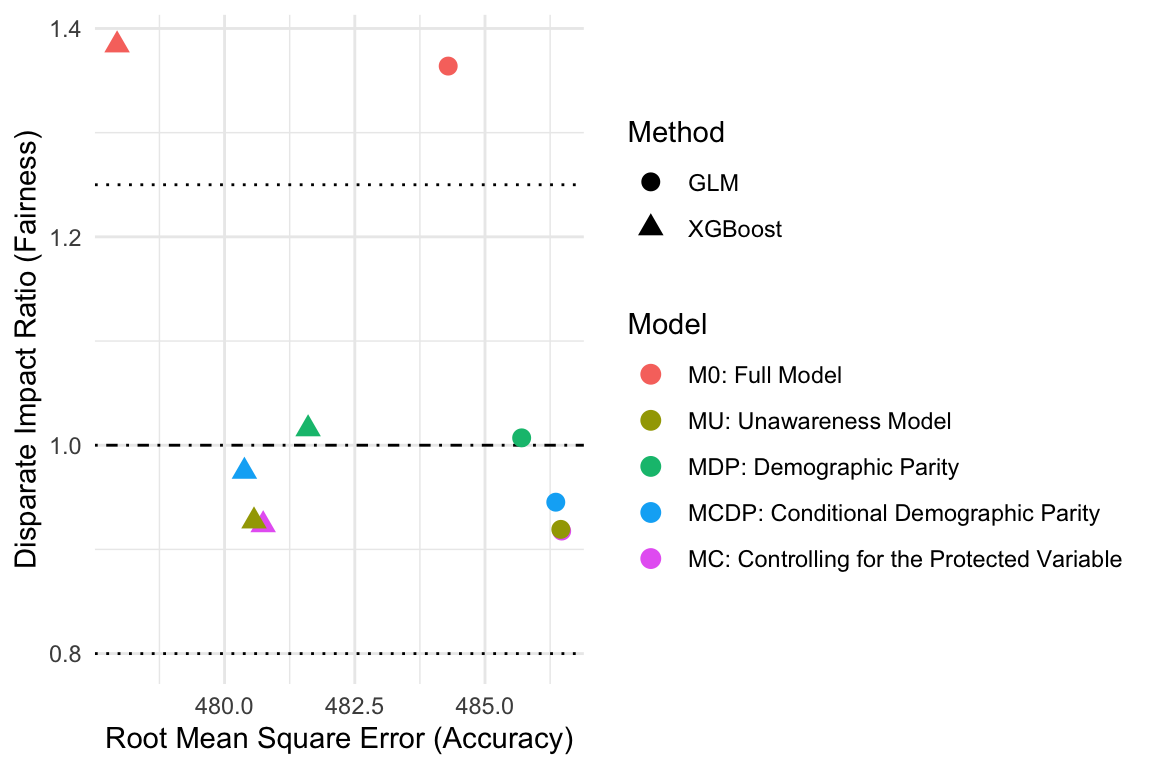
## Reading the fairness–accuracy plot
**What to look for:**
- Points near the dashed line ($\text{DIR} = 1$) are most fair.
- Points within dotted lines ($0.8$–$1.25$) satisfy the four-fifths rule.
- Points further left (lower RMSE) are more accurate.
**Key finding** [@xin2024antidiscrimination]: MCDP and MC achieve DIR close to 1 with only modest accuracy loss relative to M0. The cost of fairness is smaller than often assumed.
# Premium redistribution
## Who gains and who loses?
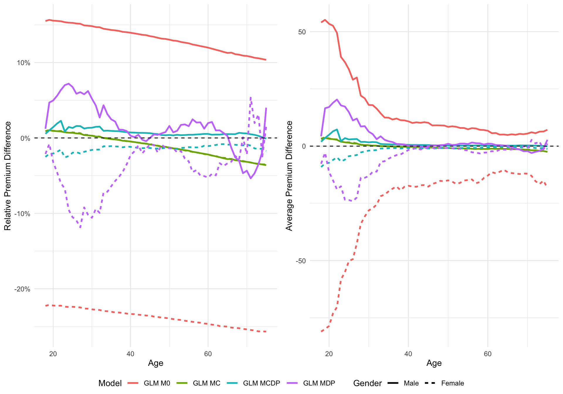
We compare each fair model to MU (the industry-standard unawareness benchmark) to show how premiums are **redistributed** across age and gender groups.
$$\text{Relative Premium Difference}_{i} = \frac{\bar{Y}_{\text{model},i} - \bar{Y}_{\text{MU},i}}{\bar{Y}_{\text{MU},i}}$$
Positive values mean the fair model charges **more** than MU for that age–gender group.
Negative values mean it charges **less** than MU.
```{r}
#| code-fold: true
#| code-summary: "Premium difference plot"
#| fig-cap: "Relative and average premium differences relative to GLM MU."
#| fig-width: 10
#| fig-height: 7
# Average predicted premium for every (age, gender) combination, one row per model.
# This is the raw material both redistribution plots below are built from.
premium_difference_by_age <- glmpred_sum %>%
  group_by(Age.ct, Gender) %>%
  summarise(`GLM M0`=mean(PurePrem1), `GLM MU`=mean(PurePrem2),
            `GLM MDP`=mean(PurePrem3), `GLM MCDP`=mean(PurePrem4),
            `GLM MC`=mean(PurePrem5), .groups="drop")

# Percentage difference from MU (the benchmark) for each age-gender group, e.g. a value
# of 0.10 means that model charges 10% more than MU for that group.
premium_difference_relative <- premium_difference_by_age %>%
  transmute(Age.ct, Gender,
    `GLM M0`  =`GLM M0`  /`GLM MU`-1, `GLM MDP` =`GLM MDP` /`GLM MU`-1,
    `GLM MCDP`=`GLM MCDP`/`GLM MU`-1, `GLM MC`  =`GLM MC`  /`GLM MU`-1) %>%
  pivot_longer(cols=-c(Age.ct,Gender), names_to="Model", values_to="Difference")

# Same idea, but as a dollar (absolute) difference from MU instead of a percentage.
premium_difference_average <- premium_difference_by_age %>%
  transmute(Age.ct, Gender,
    `GLM M0`  =`GLM M0`  -`GLM MU`, `GLM MDP` =`GLM MDP` -`GLM MU`,
    `GLM MCDP`=`GLM MCDP`-`GLM MU`, `GLM MC`  =`GLM MC`  -`GLM MU`) %>%
  pivot_longer(cols=-c(Age.ct,Gender), names_to="Model", values_to="Difference")

# Left panel: relative (%) premium difference from MU, by age and gender. The dashed
# line at 0 marks "identical to MU"; percent_format() labels the y-axis as percentages.
p_rel <- ggplot(premium_difference_relative, aes(x=Age.ct, y=Difference, colour=Model, linetype=Gender)) +
  geom_line(linewidth=1) + geom_hline(yintercept=0, linetype="dashed") +
  scale_y_continuous(labels=percent_format(accuracy=1)) +
  labs(x="Age", y="Relative Premium Difference", colour="Model", linetype="Gender") +
  guides(colour=guide_legend(order=1), linetype=guide_legend(order=2)) + theme_minimal()

# Right panel: the same comparison, but in dollar terms rather than percentage terms.
p_avg <- ggplot(premium_difference_average, aes(x=Age.ct, y=Difference, colour=Model, linetype=Gender)) +
  geom_line(linewidth=1) + geom_hline(yintercept=0, linetype="dashed") +
  labs(x="Age", y="Average Premium Difference", colour="Model", linetype="Gender") +
  guides(colour=guide_legend(order=1), linetype=guide_legend(order=2)) + theme_minimal()

ggarrange(p_rel, p_avg, common.legend=TRUE, legend="bottom")
```
## Reading the redistribution plots
- **MDP** (demographic parity): produces the clearest transfer pattern, raising premiums for the lower-charging group and lowering them for the higher-charging group across most age bands.
- **MCDP** (conditional demographic parity): stays closer to MU because legitimate variables are retained unchanged. Only the non-legitimate proxy is debiased.
- **MC** (CPV): intermediate redistribution, reflecting the gender coefficient in M0 only.
This illustrates the **solidarity principle**. Stricter fairness criteria imply more cross-subsidy between groups.
# Case study: pretrial risk assessment (COMPAS)
Consider a county criminal court system in the United States deciding whether to renew its contract for a pretrial risk-assessment tool that helps judges set bail and release conditions. The tool has been in use for several years and is credited with reducing unnecessary pretrial detention, but a recent independent audit, echoing the real-world ProPublica investigation into the actual COMPAS tool [@angwin2016machine], found that it flags Black defendants who do **not** go on to reoffend as high-risk far more often than it flags white defendants who do not reoffend. Civil-rights advocates argue the tool should be scrapped. The vendor and some judges argue it still outperforms unstructured human judgment, and that scrapping it would return the county to a less consistent, not necessarily fairer, status quo. Before the contract renewal vote, the county's Chief Public Defender has been asked to independently evaluate the tool: does it satisfy a fairness criterion the court could defend under legal challenge, and if not, can a correction be applied without making the tool too inaccurate to serve its stated purpose?
Everything in this chapter so far has been a **regression** problem: predicting a continuous price. This decision is different. It is **binary**: release or detain, flag or clear. The M0/MU model-design framework from Chapter 2 applies unchanged. Only the model type and the fairness metrics change.
We evaluate this scenario using the actual COMPAS recidivism-risk dataset (recidivism means being arrested for a new crime after release), fitting the models ourselves and using the [`fairness`](https://CRAN.R-project.org/package=fairness) R package [@kozodoi2021fairness] to compute standard classification-fairness metrics directly from group labels and predicted probabilities.
::: {.callout-tip}
The same workflow from the pricing case study applies here: fix the criterion → choose the intervention stage → fit → measure the trade-off → inspect who is affected. Only the outcome (a binary decision, not a price) and the fairness metrics change.
:::
# COMPAS: setup
```{r}
#| code-fold: true
#| code-summary: "Load the COMPAS data"
#| message: false
library(fairness)

# fairmodels (loaded above) also ships a dataset called `compas` --
# name the source package explicitly to avoid resolving the wrong one.
data(compas, package = "fairness")

# Keep only the two largest ethnicity groups; droplevels() removes the now-unused
# factor levels (e.g. "Hispanic", "Other") so they don't show up in later summaries or plots.
compas_data <- compas %>%
  filter(ethnicity %in% c("Caucasian", "African_American")) %>%
  mutate(ethnicity = droplevels(ethnicity))
```
- N = 5,278 defendants (2,103 Caucasian; 3,175 African-American), from the cleaned dataset shipped with the `fairness` package
- Response: **two-year recidivism** (`Two_yr_Recidivism`: yes/no)
- Protected attribute: **ethnicity** (Caucasian vs African-American, the two largest groups)
- Predictors: number of prior offences, two age-band indicators, gender, misdemeanour flag
Base recidivism rates already differ sharply by group, at **39.1%** (Caucasian) vs **52.3%** (African-American). This single fact turns out to drive most of what follows.
## Exploratory data analysis
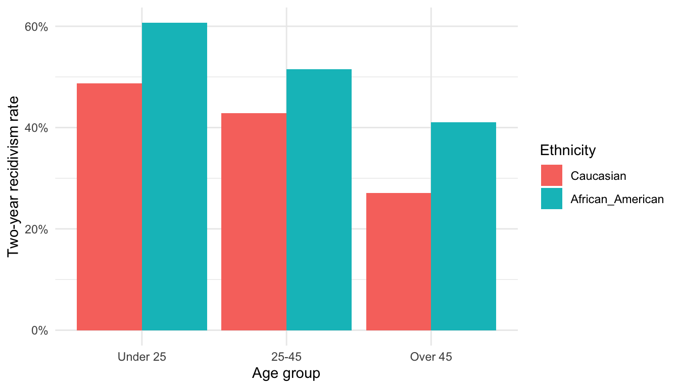
Before fitting anything, it is worth checking whether the ethnicity gap holds within subgroups too, or whether it is really an age effect in disguise.
```{r}
#| code-fold: true
#| code-summary: "Recidivism rate by ethnicity and age group"
#| fig-cap: "Two-year recidivism rate by ethnicity and age group. The gap between groups persists within every age band."
#| fig-width: 7
#| fig-height: 4
# case_when() combines the two yes/no age-band indicator columns in the data into a
# single three-level AgeGroup factor (checked top to bottom; TRUE ~ "25-45" is the
# fallback for everyone not caught by the first two conditions).
compas_eda <- compas_data %>%
  mutate(
    AgeGroup = case_when(
      Age_Below_TwentyFive == "yes" ~ "Under 25",
      Age_Above_FourtyFive == "yes" ~ "Over 45",
      TRUE ~ "25-45"
    ),
    AgeGroup = factor(AgeGroup, levels = c("Under 25", "25-45", "Over 45"))
  ) %>%
  group_by(ethnicity, AgeGroup) %>%
  # mean(Two_yr_Recidivism == "yes") is a shortcut for "proportion of TRUEs", i.e. the
  # recidivism rate within each ethnicity-age group; n() counts rows per group.
  summarise(RecidivismRate = mean(Two_yr_Recidivism == "yes"), N = n(), .groups = "drop")

# Grouped bar chart: one pair of bars per age group, one bar per ethnicity within each pair.
ggplot(compas_eda, aes(x = AgeGroup, y = RecidivismRate, fill = ethnicity)) +
  geom_col(position = "dodge") +
  scale_y_continuous(labels = scales::percent) +
  labs(x = "Age group", y = "Two-year recidivism rate", fill = "Ethnicity") +
  theme_minimal()
```
The gap holds in every age band, ranging from about 9 percentage points (25-45) to about 14 (over 45). Age alone does not explain the disparity, which is why the fairness metrics below are needed to characterise it precisely rather than relying on the raw rates.
# COMPAS: fitting the models
```{r}
#| code-fold: true
#| code-summary: "Fit M0 and MU logistic regressions"
# family = binomial fits a logistic regression: the outcome (recidivism, yes/no) is
# binary, unlike the continuous claim cost modelled with GLM above. m0 includes ethnicity
# as a predictor; mu is identical except ethnicity is left out (the M0/MU pattern from
# the pricing case study, applied here to a classification problem).
m0 <- glm(Two_yr_Recidivism ~ Number_of_Priors + Age_Above_FourtyFive + Age_Below_TwentyFive +
            Female + Misdemeanor + ethnicity, data = compas_data, family = binomial)

mu <- glm(Two_yr_Recidivism ~ Number_of_Priors + Age_Above_FourtyFive + Age_Below_TwentyFive +
            Female + Misdemeanor, data = compas_data, family = binomial)

# type = "response" returns predicted probabilities of recidivism (0 to 1), rather
# than the log-odds scale the logistic regression works in internally.
compas_data$prob_M0 <- predict(m0, type = "response")
compas_data$prob_MU <- predict(mu, type = "response")
```
M0 includes ethnicity directly. MU removes it, mirroring the actual COMPAS tool, which does not use race as an input. A defendant is flagged high-risk whenever the model's predicted probability of recidivism is above the cutoff, 0.5 here.
# COMPAS: results
## Fairness metrics with the `fairness` package
We compute three group fairness checks from Chapter 2's taxonomy for both M0 and MU. Each uses a specific `fairness` package function, and it matters exactly which statistic each one computes:
- **Demographic parity** ($\hat{Y} \perp X_P$): use `prop_parity()`, which compares each group's *proportion* positively classified. (`dem_parity()` compares *raw counts* instead, which is distorted here because the two groups have very different sizes, 2,103 vs 3,175, so it is the wrong function for this criterion.)
- **A partial check on separation**: `equal_odds()` computes group sensitivity (true-positive rate) only. This is closer to *equal opportunity* than to full equalized odds, which requires parity in both the true-positive and false-positive rate. We report FPR and FNR directly (computed manually below) to see the fuller picture.
- **A partial check on sufficiency**: `pred_rate_parity()` compares precision (positive predictive value) only, one direction of the full sufficiency condition $Y \perp X_P \mid \hat{Y}$, which also requires equal negative predictive value.
```{r}
#| code-fold: true
#| code-summary: "Compute proportional parity, equal opportunity, and predictive rate parity"
# Each fairness-package function is called twice, once per model (M0, MU), so the two
# models' disparity ratios can be compared. `base = "Caucasian"` sets the reference
# group the ratio is computed against; `cutoff = 0.5` is the probability threshold
# above which a defendant counts as "flagged high-risk".
pp_m0  <- prop_parity(data = compas_data, outcome = "Two_yr_Recidivism", outcome_base = "no",
                      group = "ethnicity", probs = "prob_M0", cutoff = 0.5, base = "Caucasian")
pp_mu  <- prop_parity(data = compas_data, outcome = "Two_yr_Recidivism", outcome_base = "no",
                      group = "ethnicity", probs = "prob_MU", cutoff = 0.5, base = "Caucasian")
eo_m0  <- equal_odds(data = compas_data, outcome = "Two_yr_Recidivism", outcome_base = "no",
                      group = "ethnicity", probs = "prob_M0", cutoff = 0.5, base = "Caucasian")
eo_mu  <- equal_odds(data = compas_data, outcome = "Two_yr_Recidivism", outcome_base = "no",
                      group = "ethnicity", probs = "prob_MU", cutoff = 0.5, base = "Caucasian")
prp_m0 <- pred_rate_parity(data = compas_data, outcome = "Two_yr_Recidivism", outcome_base = "no",
                      group = "ethnicity", probs = "prob_M0", cutoff = 0.5, base = "Caucasian")
prp_mu <- pred_rate_parity(data = compas_data, outcome = "Two_yr_Recidivism", outcome_base = "no",
                      group = "ethnicity", probs = "prob_MU", cutoff = 0.5, base = "Caucasian")
```
| Model | Accuracy | Flagged high-risk: Caucasian / African-American | FPR: Caucasian / African-American | FNR: Caucasian / African-American | Precision: Caucasian / African-American |
|-------|----------|---------------------------------------------------|-------------------------------------|-------------------------------------|--------------------------------------------|
| M0 (with ethnicity) | 66.8% | 25.1% / 52.9% | 15.9% / 35.3% | 60.7% / 31.1% | 61.3% / 68.2% |
| MU (unawareness) | 66.5% | 26.1% / 50.6% | 17.2% / 33.0% | 60.0% / 33.4% | 59.9% / 68.9% |
| Criterion | M0 disparity ratio | MU disparity ratio |
|-----------|--------------------|---------------------|
| Demographic parity (`prop_parity`) | **2.11** | **1.94** |
| Equal opportunity / TPR gap (`equal_odds`) | 1.75 | 1.67 |
| Predictive rate parity / precision gap (`pred_rate_parity`) | 1.11 | 1.15 |
## Reading the result
Unawareness barely moves anything. MU costs essentially no accuracy (66.5% vs 66.8%), but every disparity ratio survives almost unchanged whether or not the model sees ethnicity directly. An African-American defendant who will **not** reoffend is flagged high-risk roughly twice as often as a Caucasian defendant who will not reoffend (the FPR gap: 33.0% vs 17.2% under MU). This is the same qualitative finding ProPublica reported for the actual COMPAS tool [@angwin2016machine], and it replicates here on a simple logistic regression using four generic predictors.
The three checks disagree sharply on **how bad** the disparity is, and that disagreement is itself the lesson.
::: {.callout-important}
**Demographic parity shows the largest gap (ratio ≈ 2), the TPR/equal-opportunity gap is moderate (ratio ≈ 1.7), and the precision gap is comparatively small (ratio ≈ 1.1).** This is not three independent findings — it is one finding viewed through different statistics. Demographic parity ignores the true outcome entirely, so it fully reflects the underlying gap in base recidivism rates (39.1% vs 52.3%) in addition to any model unfairness. Precision conditions on the prediction, which partly absorbs that same base-rate gap. Chapter 2's Separation vs Sufficiency box showed that separation and sufficiency generally cannot both be satisfied when base rates differ, except in special cases such as perfect prediction. This is that impossibility result, observed on real data, not a theoretical curiosity. **Choosing a criterion is choosing how much of the base-rate difference counts as "unfairness" versus "signal."**
:::
Applying MDP- or MCDP-style debiasing to the predictors before fitting (exactly as in the pricing case study above) would move these ratios closer to 1, at some cost to accuracy. This is the identical trade-off already explored above, just measured in classification disparity ratios instead of a disparate impact ratio on premiums.
# COMPAS: post-processing correction
## Achieving a criterion: post-processing with `roc_pivot()`
The `fairness` package only *measures* disparity. It has no correction method. `fairmodels` (already used above for the insurance disparate-impact remover) also provides **post-processing**. `roc_pivot()` implements a reject-option correction [@kamiran2012decision], which relabels predictions that fall within a band of width `theta` around the decision cutoff, giving the disadvantaged group's borderline cases the benefit of the doubt and pulling the advantaged group's borderline cases the other way.
Mechanically, this is a mirror reflection across the cutoff: a borderline probability $p$ becomes $2 \times \text{cutoff} - p$. A privileged individual whose prediction was just barely favourable gets flipped to unfavourable; a disadvantaged individual whose prediction was just barely unfavourable gets flipped to favourable. Predictions outside the band, where the model is confident, are left untouched.
`roc_pivot()` assumes a probability above the cutoff represents the *favourable* outcome, and that `privileged` names the *privileged* group. In our model, a probability above 0.5 means predicted recidivism, the unfavourable outcome, so we convert the model to predict **non-recidivism** as the favourable outcome before calling `roc_pivot()`, keeping Caucasian (the group favoured by the status quo model) as the privileged group. This keeps the function's parameters meaning what their names say, rather than relying on two compensating reversals to get the right direction.
```{r}
#| code-fold: true
#| code-summary: "Post-process MU with roc_pivot at several theta values"
#| message: false
library(DALEX)

# Favourable outcome: no recidivism
y_favourable <- as.integer(compas_data$Two_yr_Recidivism == "no")

# Convert the fitted model's recidivism probability into a non-recidivism probability
predict_non_recidivism <- function(model, newdata) {
  1 - predict(model, newdata = newdata, type = "response")
}

# roc_pivot() (from fairmodels) doesn't work on the raw glm object directly; it needs
# a DALEX "explainer" wrapper, which bundles the model with its data, true outcome,
# and (here) a custom predict_function so roc_pivot() sees non-recidivism probabilities.
mu_explainer <- DALEX::explain(
  mu, data = compas_data, y = y_favourable,
  predict_function = predict_non_recidivism, verbose = FALSE
)

# The actual post-processing correction: relabels predictions within `theta` of the
# 0.5 cutoff, shifting borderline cases toward the outcome that favours the non-privileged
# group. Re-run this line with different `theta` values to reproduce the table below.
mu_fixed <- roc_pivot(mu_explainer, protected = compas_data$ethnicity,
                       privileged = "Caucasian", cutoff = 0.5, theta = 0.05)

# roc_pivot returns adjusted probabilities of non-recidivism;
# convert back to recidivism probabilities so downstream code keeps the original convention.
compas_data$prob_MU_fixed <- 1 - mu_fixed$y_hat
```
| theta | Accuracy | Demographic parity | Equal opportunity (TPR gap) | Predictive rate parity |
|-------|----------|---------------------|------------------------------|--------------------------|
| 0 (MU, uncorrected) | 66.5% | 1.94 | 1.67 | 1.15 |
| 0.05 | 65.7% | 1.13 | 1.11 | 1.31 |
| 0.10 | 62.8% | 0.63 | 0.69 | 1.45 |
| 0.15 | 59.4% | 0.34 | 0.40 | 1.59 |
| 0.20 | 56.8% | 0.23 | 0.30 | 1.73 |
## Reading the trade-off
At `theta = 0.05`, a modest accuracy cost (66.5% → 65.7%) buys a large improvement in demographic parity (1.94 → 1.13) and brings the TPR gap almost exactly to parity (1.67 → 1.11). That looks like a free lunch, until the predictive-rate-parity column is read alongside it.
::: {.callout-important}
**Predictive rate parity gets monotonically *worse* as the correction gets stronger**, moving from 1.15 (barely violated) to 1.73 (badly violated) as `theta` increases from 0 to 0.20. Pushing demographic parity and the TPR gap toward 1 does not leave the precision gap alone — it actively widens it. Past `theta ≈ 0.10`, demographic parity and the TPR gap **overshoot below 1**, meaning the correction has now reversed the disparity rather than closed it, at a steep accuracy cost (66.5% → 56.8%, not much better than a coin flip).
This is the Chapter 2 impossibility result, demonstrated as a dial rather than a single before/after snapshot. There is no `theta` that satisfies all three checks at once, because none exists while the two groups' base recidivism rates differ. Post-processing lets you choose *where on this curve* to sit. It does not let you escape the curve.
:::
# Summary
- All four anti-discrimination model designs can be implemented on real insurance data with modest accuracy loss, and the same workflow (fix criterion → choose stage → fit → measure trade-off → inspect redistribution) transfers to other domains, including binary classification (COMPAS, above).
- The choice of model should **follow from the regulatory criterion** chosen in Chapter 2, not from modelling convenience.
- MDP produces the strongest group fairness but the largest outcome redistribution. MCDP is more targeted.
- Unawareness (MU) is rarely sufficient on its own. The COMPAS case study shows this holding even in a binary classification setting entirely outside insurance.
- Post-processing can move a classifier toward any one group fairness check, but not all three at once. Pushing the TPR gap and demographic parity toward parity actively worsened predictive rate parity in the COMPAS example. Picking a correction method is inseparable from picking a criterion in Chapter 2's Step 1.
# Recommended reading
**Main resource**
- [fair.feihuang.org — Step 2: Design Fair Pricing](https://fair.feihuang.org/Playbook/Step-2-Design-Fair-Pricing.html) and its linked [Case Study: Fair Models](https://fair.feihuang.org/Case%20Study%202/case_study2.html), the full technical write-up this lecture walks through
**Further reading**
- @xin2024antidiscrimination, source paper for all five model designs and the fairness–accuracy analysis
- @barocas2023fairml, [*Fairness and Machine Learning: Limitations and Opportunities*](https://fairmlbook.org), freely available online. Chapter 3 ("Regression") extends the classification-based criteria in Chapter 2 to continuous outcomes like pure premium, and Chapter 2 ("Classification") covers the criteria used in the COMPAS case study
- @lindholm2022discrimination, discrimination-free pricing and the CPV (MC) approach
- @feldman2015certifying, disparate-impact remover algorithm
- @angwin2016machine, the original COMPAS investigation behind the binary classification case study above
- @kozodoi2021fairness, the `fairness` R package used for demographic parity, equalized odds, and predictive rate parity
- @kamiran2012decision, the reject-option post-processing method behind `roc_pivot()`