---
title: "Privacy Practice"
urlcolor: blue
bibliography: reference.bib
resources:
- "data/pg15training_raw.csv"
other-links:
- text: In-class slides
href: Slides-Privacy-Practice.slides.html
icon: easel2
format:
html:
code-tools: true
code-fold: true
format-links: false
pdf:
documentclass: article
pdf-engine: xelatex
toc: true
toc-depth: 3
geometry: margin=0.6in
fontsize: 9pt
colorlinks: true
include-in-header:
text: |
\usepackage{fvextra}
\fvset{breaklines,breakanywhere}
execute:
echo: true
warning: false
message: false
---
## Learning objectives
- Conduct a basic privacy risk assessment for a tabular dataset by identifying quasi-identifiers and measuring re-identification risk.
- Apply k-anonymity and assess re-identification risk using real data.
- Implement the Laplace mechanism for differentially private statistics.
- Generate and evaluate synthetic data as an alternative to releasing real records.
- Measure the privacy–utility trade-off for each technique and identify appropriate controls for each stage of the data lifecycle.
## From principle to practice
Chapter 6 introduced *why* a dataset carries re-identification risk and *which* privacy-enhancing technique (PET) addresses it. Turning that choice into a working pipeline follows the same sequence regardless of domain:
1. **Identify quasi-identifiers** (variables that are not identifying alone but can combine to reveal who someone is) in the dataset and assess re-identification risk against them.
2. **Choose a PET matched to the use case**, using suppression/generalisation (k-anonymity) for micro-data release, noise injection (differential privacy) for aggregate statistics, or synthetic generation for realistic but non-real records.
3. **Apply the technique** to the dataset.
4. **Measure the trade-off**, weighing utility loss (e.g. bias in downstream statistics or model performance) against residual disclosure risk, not one in isolation.
5. **Decide whether the trade-off is acceptable** for the intended release or use, and document the decision.
This lecture works through steps 3–5 in full, on a single worked example, so each step above has a concrete implementation to point to.
## Case study: privacy-enhancing techniques for insurance micro-data
This lecture uses the same French motor insurance dataset (`pg15training`) from Chapter 3. We use insurance data as the case study for continuity with that dataset, and because policy-level micro-data (data with one row per individual policy, rather than aggregated summaries) carries the kind of realistic quasi-identifiers, age, location, vehicle value, that make re-identification risk concrete rather than abstract. The same workflow applies to health records, HR/employment data, financial or credit data, and government census-style micro-data. We treat the dataset as a **sensitive dataset** and apply three privacy-enhancing technologies in sequence:
| Section | Method | Tool |
|---------|--------|------|
| 1. Re-identification risk | Quasi-identifier analysis | `sdcMicro` |
| 2. k-Anonymity | Generalisation and suppression | `sdcMicro` |
| 3. Differential privacy | Laplace mechanism | Base R |
| 4. Synthetic data | CART-based synthesis | `synthpop` |
```{r packages}
#| code-fold: true
#| code-summary: "Package setup"
library(sdcMicro)    # k-anonymity, local suppression, re-identification risk
library(synthpop)    # CART-based synthetic data generation
library(tidyverse)   # data wrangling and plotting
library(ggpubr)      # ggarrange() for combining multiple plots
library(scales)      # percent()/comma() formatting for tables and axes
library(knitr)       # kable() for tables
library(kableExtra)  # kable_styling() and related table formatting

set.seed(42)  # for reproducibility of sampling and Laplace noise draws below
```
# Data preparation
## The French motor insurance dataset
We use `pg15training`, originally distributed via the `CASdatasets` R package, which contains 100,000 third-party liability motor policies (car insurance contracts covering damage or injury the driver causes to others, not the driver's own vehicle) from France (2009–2010). A CSV export ([`data/pg15training_raw.csv`](data/pg15training_raw.csv)) is provided alongside this chapter, so reproducing the code below does not require installing `CASdatasets`.
The same insurer now wants to share its policy-level data externally. Getting this wrong risks a data-protection breach and undermines the customer trust that the fairness and explainability work in Chapters 3 and 5 was meant to protect.
::: {.callout-note title="Case study: deciding how to release policy data to three different recipients"}
The insurer's data governance policy requires the Head of Data Governance to sign off on any external release of policy-level data, following a documented risk assessment, the kind of process Chapter 6 introduced as a data protection impact assessment (DPIA). Three requests have arrived at once, and each has a different risk profile:
1. **A reinsurer**, pricing next year's quota-share treaty renewal, wants policy-level exposure and claims data to build its own independent pricing model. It is a repeat business partner that has audited some of the same policyholders in prior treaty years, so it may already hold partial background knowledge about who is in this portfolio, not a blind outsider starting from zero.
2. **The insurer's own actuarial pricing team**, building next year's rating model, needs data that behaves like the real portfolio, realistic correlations, realistic rare combinations, but the model will be validated against the live production system regardless, so it does not strictly need the actual individual records.
3. **An industry benchmarking vendor**, building a market-wide rate comparison tool for a regulator's market-conduct review, needs aggregate statistics by rating factor, not individual policy records at all.
The Head of Data Governance must decide, for each recipient, which privacy-enhancing technique, if any, is proportionate, and document that decision before any data leaves the building.
**Questions to consider as you work through this chapter:**
- Which of the three recipients could the insurer defensibly hand k-anonymised data to, and which would need a stronger technique? Does the reinsurer's partial background knowledge change your answer, given what Chapter 6 already said about recipients who are not blind outsiders?
- The pricing team does not strictly need real records, only realistic ones. Does that argue for synthetic data specifically, or is there a simpler, cheaper answer available given the team is internal?
- The vendor only needs aggregate statistics, not a record-level file at all. Does that change which of this chapter's three techniques is even the relevant one for that request?
We will return to this case study once all three techniques have been applied to this dataset, with actual measured numbers to answer these questions rather than intuition alone.
:::
All three use cases raise privacy questions, even though names and policy numbers are absent.
```{r data-prep}
#| code-fold: true
#| code-summary: "Data preparation"
pg15training <- read.csv("data/pg15training_raw.csv", stringsAsFactors = TRUE)

# Remove the 21 duplicate records as in Chapter 3
df_raw <- pg15training %>%
  slice(-(1:21)) %>%
  mutate(
    Gender    = as.factor(Gender),
    Group1    = as.factor(Group1),
    Bonus     = as.factor(Bonus),
    # Group continuous variables into bands for quasi-identifier analysis.
    # Banding is itself a mild form of generalisation/anonymisation: exact
    # values are already hidden before k-anonymity is applied below.
    AgeGroup  = cut(Age,
                    breaks = c(17, 25, 35, 45, 55, 65, Inf),
                    labels = c("18-25","26-35","36-45","46-55","56-65","66+")),
    DensityGroup = cut(Density,
                       breaks = c(0, 50, 100, 200, Inf),
                       labels = c("Rural","Suburban","Urban","Dense urban")),
    ValueGroup = cut(Value,
                     breaks = c(0, 5000, 15000, 30000, Inf),
                     labels = c("Low","Medium","High","Luxury")),
    BonusGroup = cut(as.numeric(Bonus),
                     breaks = c(0, 3, 7, 11, Inf),
                     labels = c("Low","Medium","High","Very high")),
    HasClaim  = as.integer(Numtppd > 0),  # 1 if the policy had at least one claim, else 0
    ClaimAmount = Indtppd                 # amount paid out (0 if no claim)
  )

cat("Dataset: ", nrow(df_raw), "policies\n")
cat("Variables:", ncol(df_raw), "\n")
```
## What does "anonymised" look like?
Suppose we strip direct identifiers and share this dataset for research. What remains looks like:
```{r show-sample}
#| results: asis
# Keep only fields a data-sharing agreement might allow through; no name,
# policy number, or exact address, just what looks like an "anonymised" extract
df_raw %>%
  select(Gender, Age, AgeGroup, DensityGroup, ValueGroup, BonusGroup, HasClaim, ClaimAmount) %>%
  slice(1:6) %>%
  kable(caption = "First six records after removing direct identifiers") %>%
  kable_styling(font_size = 11)
```
`HasClaim` flags whether the policyholder filed an insurance claim (a request for payment after an accident), and `ClaimAmount` is how much was paid out.
At first glance this looks anonymous. But is it?
# Re-identification risk assessment
## Quasi-identifiers
**Quasi-identifiers** are variables that are not direct identifiers but can be combined to uniquely identify individuals by cross-referencing with external data.
In motor insurance data, plausible quasi-identifiers include:
| Variable | Why it's a quasi-identifier |
|----------|---------------------------|
| Gender | Combined with other variables, narrows the group substantially |
| Age (or AgeGroup) | One of the most identifying variables |
| DensityGroup | Population density of the area where the car is kept, a proxy for postcode / location, which can be cross-referenced |
| ValueGroup | Vehicle value narrows the pool, especially at extremes |
| BonusGroup | No-claims bonus level (a discount tier based on years without a claim) that narrows the pool within age group |
## Measuring re-identification risk with `sdcMicro`
`sdcMicro` [@templ2017statistical] implements standard statistical disclosure control methods. The key metric is the **individual re-identification risk**, the probability that a given record can be matched to a real individual. The **global risk** summarises this across the whole dataset, roughly the overall share of records that could plausibly be re-identified.
**How this risk is estimated.** For each record, `sdcMicro` first counts its **sample frequency** $f_k$: the number of records in the dataset, including itself, that share its exact combination of key-variable values (the equivalence class introduced above). A record unique on the key variables has $f_k = 1$.
If the file were the entire population rather than a sample of it, the probability of correctly guessing a target's identity among $f_k$ indistinguishable records is simply
$$
r_k = \frac{1}{f_k}.
$$
`sdcMicro`'s default estimator generalises this: because a released file is often only a sample of a larger population, it models the relationship between the sample frequency $f_k$ and the unknown population frequency using a super-population model, assuming a negative binomial distribution for how sample counts relate to population counts [@franconi2004individual]. No sampling weight is supplied to `createSdcObj()` below, so the file is effectively treated as the population, and the estimate reduces toward the simple $1/f_k$ intuition above: rarer combinations carry proportionally higher risk.
This is the direct mathematical link to the next section. **k-anonymity requires every equivalence class to contain at least $k$ records**, that is $f_k \geq k$ for every record, which is exactly the guarantee $r_k \leq 1/k$.
**Global risk and expected re-identifications.** Summing the individual risk $r_k$ across every record gives the **expected number of re-identifications**, how many records an attacker would successfully match, in expectation, if they tried to re-identify every record from its key variables. Global risk expresses this same total as a share of the dataset, the expected number of re-identifications divided by the number of records.
```{r sdc-object}
#| code-fold: true
#| code-summary: "Create sdcMicro object"
# Restrict to the columns relevant for disclosure control: quasi-identifiers
# plus one sensitive numeric variable (ClaimAmount) whose risk we also track
df_sdc <- df_raw %>%
  select(Gender, AgeGroup, DensityGroup, ValueGroup, BonusGroup,
         HasClaim, ClaimAmount) %>%
  as.data.frame()

# createSdcObj() computes, among other things, each record's sample frequency
# f_k and individual risk r_k (see the r_k = 1/f_k discussion above), from
# just the keyVars combination each record falls into
sdc <- createSdcObj(
  dat     = df_sdc,
  keyVars = c("Gender", "AgeGroup", "DensityGroup", "ValueGroup", "BonusGroup"),
  numVars = c("ClaimAmount")
)
```
```{r risk-summary}
#| results: asis
risk_global <- sdc@risk$global
# sdc@risk$individual column 2 holds each record's equivalence-class size f_k
k_counts <- table(sdc@risk$individual[, 2])

tibble(
  Metric = c("Global re-identification risk",
             "Expected number of re-identifications",
             "Maximum individual risk",
             "Records with k = 1 (unique)",
             "Records with k <= 3",
             "Records with k <= 5"),
  Value = c(
    percent(risk_global$risk, accuracy = 0.01),
    round(risk_global$risk_ER, 0),
    round(max(sdc@risk$individual[, "risk"]), 4),  # highest r_k in the dataset
    sum(sdc@risk$individual[, 2] == 1),  # f_k = 1: unique on the 5 quasi-identifiers
    sum(sdc@risk$individual[, 2] <= 3),
    sum(sdc@risk$individual[, 2] <= 5)
  )
) %>%
  kable(caption = "Re-identification risk summary (5 quasi-identifiers)") %>%
  kable_styling(font_size = 12)
```
## Interpreting the risk
The global risk is low because the dataset is large (100,000 records) and the quasi-identifiers are already grouped into broad bands.
But this understates the real risk. In practice:
- A reinsurer receiving this data may **already know** which policyholders (the people who hold the policies) are in the portfolio. They only need to confirm details, not identify from scratch
- An attacker with access to vehicle registration data could cross-reference **ValueGroup** and **AgeGroup** to narrow candidates dramatically
- **Rare combinations** (e.g. "66+, Dense urban, Luxury vehicle, Low bonus") are highly re-identifiable even in a large dataset
```{r rare-combos}
#| results: asis
# Group by every quasi-identifier combination and count records per group
# (this group size is exactly the f_k discussed above); the smallest groups
# are the ones an attacker could most easily narrow down to one individual
df_sdc %>%
  count(Gender, AgeGroup, DensityGroup, ValueGroup, BonusGroup, name = "n_records") %>%
  filter(n_records <= 5) %>%
  arrange(n_records) %>%
  slice(1:10) %>%
  kable(caption = "Ten smallest quasi-identifier groups (highest re-identification risk)") %>%
  kable_styling(font_size = 11)
```
## The aggregation problem
Each quasi-identifier alone is innocuous:
- Knowing someone is male is not identifying
- Knowing someone is in the 66+ age group is not identifying
- Knowing someone has a luxury vehicle is not identifying
**Combined**, these three variables dramatically narrow the pool. This is Solove's **aggregation** problem from Chapter 6.
```{r aggregation-demo}
#| results: asis
# Count how many records remain as each additional quasi-identifier filter is
# stacked on top of the previous ones, to show the anonymity set shrinking
df_raw %>%
  summarise(
    `All records`                     = n(),
    `Male only`                       = sum(Gender == "Male"),
    `Male, 66+`                       = sum(Gender == "Male" & AgeGroup == "66+"),
    `Male, 66+, Luxury vehicle`       = sum(Gender == "Male" & AgeGroup == "66+" &
                                             ValueGroup == "Luxury"),
    `Male, 66+, Luxury, Dense urban`  = sum(Gender == "Male" & AgeGroup == "66+" &
                                             ValueGroup == "Luxury" &
                                             DensityGroup == "Dense urban")
  ) %>%
  pivot_longer(everything(), names_to = "Filter", values_to = "Records remaining") %>%
  kable(caption = "How combination of quasi-identifiers reduces the anonymity set") %>%
  kable_styling(font_size = 12)
```
The **anonymity set** here is the group of records that share the same quasi-identifier values, the pool a person could hide in. As filters stack up, that pool shrinks toward a single record.
# k-Anonymity
## Applying k-anonymity with `sdcMicro`
The quasi-identifiers above were already **generalised** into bands during data preparation (exact age into age band, exact density into density band, and so on). A dataset satisfies **k-anonymity** if every combination of quasi-identifier values shared by at least one record is shared by at least $k$ records in total, that is, each record's equivalence class contains the record itself plus at least $k - 1$ others. Generalisation alone still leaves many equivalence classes far below the $k = 50$ enforced below, including groups as small as a single record, as the "Ten smallest quasi-identifier groups" table above already showed.
This section applies **local suppression**, where records in groups smaller than $k$ have their most identifying quasi-identifier values suppressed (set to `NA`), on top of the existing bands, to bring every remaining group up to $k$. We use $k = 50$ here, larger than the $k = 5$ textbook minimum, precisely so the suppression and its utility cost are visible rather than marginal: with only 102 records below $k = 5$ out of 100,000, a $k = 5$ pass barely touches the dataset.
**How local suppression decides what to suppress.** For each record whose equivalence class is smaller than $k$, `localSuppression()` searches for the smallest number of quasi-identifier values it can convert to missing to bring that record's class up to size $k$, using the `importance` vector to decide which variables to sacrifice first. A **lower** importance value protects a variable from suppression; a **higher** value marks it for suppression first. The code below ranks `Gender` as most protected (`importance = 1`) and `BonusGroup` as most disposable (`importance = 5`), following the order of `keyVars`. This is a judgement call: Gender is a rating factor several regulators restrict or scrutinise (Chapters 2-3), so it is worth protecting from suppression even at the cost of losing more information from `BonusGroup` when a record needs it.
```{r kanonymity}
#| code-fold: true
#| code-summary: "Apply k = 50 anonymisation"
# k = 50 (not the textbook-minimum k = 5) so the suppression is large enough to see
sdc_k50 <- localSuppression(sdc, k = 50, importance = c(1, 2, 3, 4, 5))

risk_after <- sdc_k50@risk$global   # global risk after suppression, for comparison to `sdc` (before)

cat("Before: global risk", round(sdc@risk$global$risk_pct, 3), "%\n")
cat("After: global risk", round(risk_after$risk_pct, 3), "%\n")
cat("Suppressed cells:", sum(is.na(sdc_k50@manipKeyVars)), "\n")
```
```{r kanon-summary}
#| results: asis
# Count how many values were suppressed (set to NA) in each quasi-identifier column
suppressed <- sapply(names(sdc_k50@manipKeyVars), function(v) {
  sum(is.na(sdc_k50@manipKeyVars[[v]]))
})

tibble(
  `Quasi-identifier` = names(suppressed),
  `Suppressed values` = suppressed,
  `Suppression rate` = percent(suppressed / nrow(df_sdc), accuracy = 0.01)
) %>%
  kable(caption = "Suppression applied per quasi-identifier (k = 50)") %>%
  kable_styling(font_size = 12)
```
**Reading the result.** Global risk falls from 0.77% to 0.41%, a reduction of about 47%, roughly halving the expected number of re-identifications. All the suppression lands on `BonusGroup` and, once that stops being enough on its own, `ValueGroup`. `Gender`, `AgeGroup`, and `DensityGroup` stay untouched throughout, exactly as the `importance` ranking intended: the algorithm always exhausts the cheapest (highest-importance-number) variable before it starts spending a more protected one. This is also why a small $k$ produced almost no suppression earlier: at $k = 5$ only 102 records needed any suppression at all, and `localSuppression()` could fix nearly all of them by clearing a single `BonusGroup` value, well under 0.1% of that column. Pushing $k$ higher forces progressively more equivalence classes to merge, which is why the suppression rate accelerates rather than growing in proportion to $k$.
## The utility cost of k-anonymity
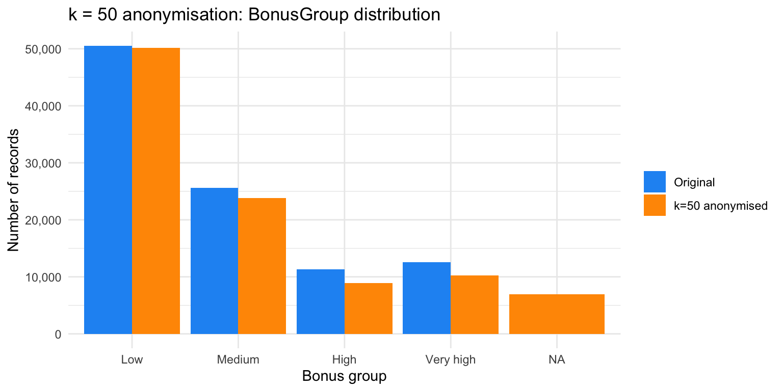
Suppression makes the data less useful. How much? The chart below uses `BonusGroup`, the variable that actually absorbs the suppression, rather than `AgeGroup` or `Gender`, which are untouched at this $k$ and would show no visible difference at all.
```{r kanon-utility}
#| fig-cap: "BonusGroup distribution before and after k=50 anonymisation. Suppressed records are shown as NA."
#| fig-width: 8
#| fig-height: 4
# "Before": the original BonusGroup distribution
before <- df_sdc %>%
  count(BonusGroup, name = "n") %>%
  mutate(Dataset = "Original")

# "After": the BonusGroup distribution once suppression has replaced some values with NA
# count() keeps NA as its own bar by default, so suppressed records appear as a visible "NA" category
after_data <- sdc_k50@manipKeyVars %>%
  as.data.frame() %>%
  count(BonusGroup, name = "n") %>%
  mutate(Dataset = "k=50 anonymised")

bind_rows(before, after_data) %>%
  ggplot(aes(x = BonusGroup, y = n, fill = Dataset)) +
  geom_col(position = "dodge") +
  scale_y_continuous(labels = comma) +
  labs(x = "Bonus group", y = "Number of records",
       fill = NULL, title = "k = 50 anonymisation: BonusGroup distribution") +
  theme_minimal() +
  scale_fill_manual(values = c("Original" = "#2196F3", "k=50 anonymised" = "#FF9800"))
```
The new `NA` bar is the utility cost made visible: 6,901 records, 6.9% of the portfolio, lose their `BonusGroup` value entirely. A downstream analyst computing claim frequency by bonus tier would now be working with a `BonusGroup` column that is systematically missing exactly the records that were hardest to protect, disproportionately the smallest, most identifying equivalence classes rather than a random sample. That is the trade-off k-anonymity forces: the records with the most disclosure risk are also the ones whose information is most degraded by the fix.
::: {.callout-note}
k-Anonymity is effective for small datasets or when sharing fine-grained geographic data. For large insurance datasets with many variables, suppression rates are low at the textbook-minimum $k = 5$, but rise quickly as $k$ increases, as shown above. The method also cannot handle continuous variables well, and **does not protect sensitive values** (the claims column is untouched).
:::
# Differential privacy
## The Laplace mechanism
Differential privacy [@dwork2006calibrating] adds calibrated noise to statistics before release, ensuring that the output reveals almost nothing about any individual record.
For a numeric function $f(D)$ with global **sensitivity** $\Delta f$ (the most a single record could change the statistic if it were added or removed, a different meaning of "sensitive" from the confidential data discussed elsewhere in this chapter), the **Laplace mechanism** releases:
$$\mathcal{M}(D) = f(D) + \text{Lap}\!\left(\frac{\Delta f}{\varepsilon}\right)$$
Here $\varepsilon$ (epsilon) is the **privacy budget**: a smaller $\varepsilon$ adds more noise and gives stronger privacy, a larger $\varepsilon$ adds less noise and gives more accurate but less private results. `Lap()` draws the noise itself from a Laplace distribution, a symmetric, bell-like curve centred on zero.
We implement this from scratch to build intuition.
```{r dp-functions}
#| code-fold: true
#| code-summary: "Differential privacy helper functions"
# Draw a single noise value from Laplace(0, sensitivity/epsilon) using the
# inverse-CDF (quantile) method: if u ~ Uniform(0,1), then
# -b * sign(u - 0.5) * log(1 - 2|u - 0.5|) is Laplace(0, b) distributed.
laplace_noise <- function(sensitivity, epsilon, n = 1) {
  scale <- sensitivity / epsilon
  u <- runif(n) - 0.5
  -scale * sign(u) * log(1 - 2 * abs(u))
}

# Differentially private mean of x, where x is known to lie in [lower, upper].
# Sensitivity of a mean over n bounded values is (upper - lower) / n: swapping
# one record can move the mean by at most one value's range, divided by n.
# This is the key reason DP noise shrinks as the group being averaged grows.
dp_mean <- function(x, lower, upper, epsilon) {
  n <- length(x)
  sensitivity <- (upper - lower) / n
  true_mean <- mean(x, na.rm = TRUE)
  true_mean + laplace_noise(sensitivity, epsilon)
}

# Differentially private count of records satisfying `condition`.
# Sensitivity of a count is 1: adding or removing one record changes the
# count by at most 1, regardless of n, so count noise does NOT shrink with n.
dp_count <- function(x, condition, epsilon) {
  true_count <- sum(condition(x), na.rm = TRUE)
  round(true_count + laplace_noise(sensitivity = 1, epsilon = epsilon))
}

# Differentially private proportion: release the count with DP, then divide
# by the (public, non-private) sample size n. Because count noise has a fixed
# scale, dividing by a small n can swing the resulting proportion a lot.
dp_proportion <- function(x, condition, epsilon) {
  n <- length(x)
  dp_count(x, condition, epsilon) / n
}
```
## DP statistics on the motor dataset
We release three statistics from the portfolio with varying privacy levels:
```{r dp-results}
#| results: asis
epsilons <- c(0.1, 0.5, 1, 5, 10)   # from very private (0.1) to almost no privacy (10)

true_mean_age    <- mean(df_raw$Age)
true_claim_rate  <- mean(df_raw$HasClaim)
true_mean_amount <- mean(df_raw$ClaimAmount[df_raw$ClaimAmount > 0])

# One DP release per epsilon, on the full 100,000-record portfolio
results <- map_dfr(epsilons, function(eps) {
  tibble(
    epsilon             = eps,
    `True mean age`     = round(true_mean_age, 2),
    `DP mean age`       = round(dp_mean(df_raw$Age, lower = 18, upper = 100, epsilon = eps), 2),
    `True claim rate`   = round(true_claim_rate, 4),
    `DP claim rate`     = round(dp_proportion(df_raw$HasClaim,
                                              condition = function(x) x == 1,
                                              epsilon = eps), 4)
  )
})

results %>%
  kable(caption = "Differentially private statistics at varying epsilon values") %>%
  kable_styling(font_size = 11)
```
**Reading this table.** Every row looks almost identical, including at $\varepsilon = 0.1$, the strictest privacy setting here. This is not a bug. With $n = 100{,}000$, the mean-age sensitivity is $(100-18)/100{,}000 \approx 0.0008$, so even the largest noise draw in this table is a fraction of a year. Large aggregates are close to "free" to protect with DP. The next section shows what happens to the same mechanism, at the same epsilon values, once the group being summarised is small rather than large.
## The privacy–utility trade-off visualised
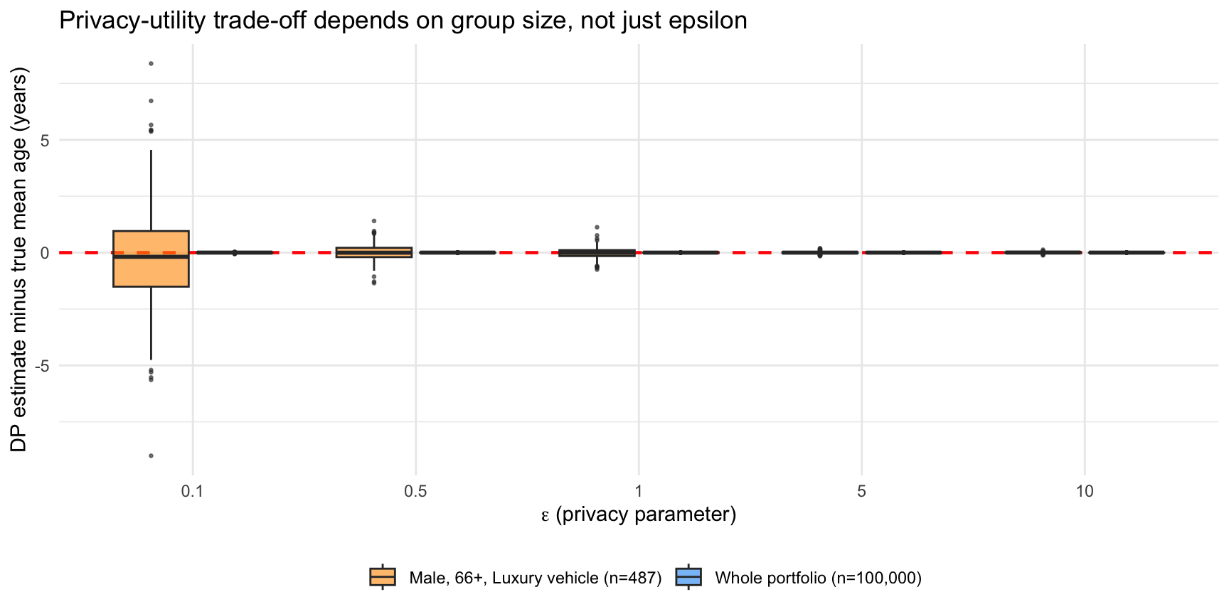
Sensitivity scales as $1/n$, so the same $\varepsilon$ produces very different amounts of noise depending on how large the group being summarised is. To make this concrete, we compare the whole 100,000-record portfolio against a small subgroup already used earlier in this lecture: **Male, 66+, Luxury vehicle** (`n = 487`, from the aggregation-problem table above).
```{r dp-tradeoff-plot}
#| fig-cap: "Variability of DP mean age estimates across 200 repeated releases at each epsilon, whole portfolio (n=100,000) vs. a small subgroup (n=487)."
#| fig-width: 9
#| fig-height: 4.5
# The same rare subgroup introduced in the aggregation-problem section above
rare_group <- df_raw %>%
  filter(Gender == "Male", AgeGroup == "66+", ValueGroup == "Luxury")

true_mean_rare <- mean(rare_group$Age)

# For each epsilon, draw 200 independent DP releases and record how far each
# one lands from the true mean, so both groups can share a common y-axis
# ("deviation from true mean") despite having different true means (~41 vs ~70)
dp_simulation <- map_dfr(epsilons, function(eps) {
  whole_estimates <- replicate(200, dp_mean(df_raw$Age, lower = 18, upper = 100, epsilon = eps))
  rare_estimates  <- replicate(200, dp_mean(rare_group$Age, lower = 18, upper = 100, epsilon = eps))
  bind_rows(
    tibble(epsilon = factor(eps), deviation = whole_estimates - true_mean_age,
           Group = "Whole portfolio (n=100,000)"),
    tibble(epsilon = factor(eps), deviation = rare_estimates - true_mean_rare,
           Group = "Male, 66+, Luxury vehicle (n=487)")
  )
})

ggplot(dp_simulation, aes(x = epsilon, y = deviation, fill = Group)) +
  geom_hline(yintercept = 0, colour = "red", linetype = "dashed", linewidth = 0.8) +
  geom_boxplot(alpha = 0.6, outlier.size = 0.5) +
  labs(x = expression(epsilon ~ "(privacy parameter)"),
       y = "DP estimate minus true mean age (years)",
       fill = NULL,
       title = "Privacy-utility trade-off depends on group size, not just epsilon") +
  theme_minimal() +
  theme(legend.position = "bottom") +
  scale_fill_manual(values = c("Whole portfolio (n=100,000)" = "#2196F3",
                                "Male, 66+, Luxury vehicle (n=487)" = "#FF9800"))
```
**Reading this plot.** The whole-portfolio boxes stay pinned to zero deviation at every $\varepsilon$, invisibly thin at this scale, echoing the table above. The small-subgroup boxes tell a different story: at $\varepsilon = 0.1$, individual releases can land more than two years off the true mean, and the box only tightens to sub-year accuracy once $\varepsilon$ reaches 5 or 10. The mechanism and the privacy budget are identical in both cases; only $n$ differs, by a factor of about 200. This is why a portfolio-wide statistic is close to free to protect with DP, while the same $\varepsilon$ applied to a fine-grained breakdown, a single postcode, a rare demographic combination, a small branch office, can add real distortion. It is also why the 2018 US Census reconstruction attack (Chapter 6) was hardest to defend against at the smallest published geographies (census blocks), not at state or national level.
## Interpreting the epsilon trade-off
| ε | Noise added to mean age (whole portfolio) | Noise added to mean age (rare subgroup, n=487) | Practical interpretation |
|---|------------------------|------------------------|--------------------------|
| 0.1 | Negligible | Very large (multi-year swings) | Strong privacy; unusable for small-group statistics, fine for portfolio-wide ones |
| 0.5 | Negligible | Large | Still risky for granular reporting |
| 1 | Negligible | Moderate | Common default, used by some regulatory frameworks |
| 5 | Negligible | Small | Acceptable even for moderately small groups |
| 10 | Negligible | Very small | Weak privacy, close to undisturbed output |
::: {.callout-note}
With $n = 100{,}000$ records, the sensitivity of the mean age is $(100-18)/100{,}000 \approx 0.0008$, so **large datasets make DP much more practical**: even at $\varepsilon = 0.1$, portfolio-wide noise is negligible. But the same guarantee costs real accuracy once $n$ is small, as the $n = 487$ subgroup above shows. Choosing $\varepsilon$ is therefore inseparable from deciding how granular a release is allowed to be.
:::
## DP claim rate by gender
We can also release group-level statistics with DP, relevant for fairness reporting. Male and Female policyholders are both large groups here (tens of thousands of records each), so, following the pattern established above, expect the DP columns to stay close to the true rate rather than swing the way the `n = 487` subgroup did:
```{r dp-gender}
#| results: asis
# Female/Male are large subgroups (tens of thousands each), unlike the n=487
# example above, so DP noise should again be small relative to the true rate
gender_dp <- map_dfr(c("Female", "Male"), function(g) {
  x <- df_raw %>% filter(Gender == g) %>% pull(HasClaim)
  tibble(
    Gender = g,
    n = length(x),
    `True claim rate` = round(mean(x), 4),
    `DP claim rate (ε=1)` = round(dp_proportion(x, function(v) v == 1, epsilon = 1), 4),
    `DP claim rate (ε=5)` = round(dp_proportion(x, function(v) v == 1, epsilon = 5), 4)
  )
})

gender_dp %>%
  kable(caption = "DP claim rate by gender — protecting group-level statistics") %>%
  kable_styling(font_size = 12)
```
As expected, both DP columns stay close to the true rate: Male and Female are large enough subgroups that even $\varepsilon = 1$ adds little noise. A regulator asking for the same breakdown by a much finer category, say claim rate by postcode, would land in the same small-$n$, large-noise regime as the rare subgroup above, and might need a larger $\varepsilon$, a coarser geography, or a different technique such as k-anonymity or synthetic data.
::: {.callout-important}
A single DP release consumes privacy budget ε. If you release multiple statistics from the same dataset, privacy budget must be **composed**. Sequential releases multiply risk. For $k$ independent queries each at $\varepsilon$, the total budget is $k\varepsilon$ (basic composition). More sophisticated accountants (e.g. Rényi DP) allow tighter bounds.
:::
# Synthetic data
## Generating synthetic insurance data with `synthpop`
`synthpop` [@nowok2016synthpop] generates **synthetic data** (artificial records that statistically resemble the real data without being any real person's actual record) by fitting a sequence of conditional models, one variable at a time, conditioning on previously synthesised variables. By default it uses CART (Classification and Regression Trees, a method that predicts each variable by repeatedly splitting the data into groups based on the other variables).
**Desired properties of synthetic data.** Synthetic data generators are judged against three properties, which do not automatically move together [@jordon2022synthetic]:
- **Fidelity**: how closely the synthetic data's distribution resembles the real data's, marginally (each variable on its own) and jointly (the relationships between variables). The marginal-distribution and summary-statistics checks below test this directly.
- **Utility**: whether the synthetic data actually supports the downstream task it was made for, not just whether it looks similar. Coefficient agreement, and more directly the train-synthetic-test-real (TSTR) check, below test this.
- **Privacy**: whether releasing the synthetic data leaks information about specific real individuals. The nearest-neighbour distance check below tests this, though a complete privacy evaluation also needs membership-inference and attribute-inference testing, discussed further below.
These three properties trade off against each other. A generator that memorised the training data would score perfectly on fidelity and utility but fail privacy completely. A generator that added so much noise or regularisation that no real record could ever be inferred would score well on privacy but poorly on fidelity and utility. The checks below test the three properties in the order a data custodian would typically need to satisfy them, fidelity first, then utility, then privacy: a synthetic dataset that does not even resemble the real data is not worth testing further.
We synthesise a working subset of the motor portfolio, holding back a slice of **real** records that `synthpop` never sees. That held-out set is not needed for the fidelity checks below, but it is essential later for testing whether a model trained on synthetic data still works on genuinely new, real records.
```{r synthpop-gen}
#| code-fold: true
#| code-summary: "Prepare synthesis dataset"
# Use the raw (not banded) variables here, since synthesis should reproduce
# realistic continuous values, not the coarser bands used for k-anonymity
df_synth_pool <- df_raw %>%
  select(Gender, Age, Group1, Bonus, Density, Value,
         Numtppd, Indtppd) %>%
  mutate(
    Group1 = as.numeric(as.character(Group1)),  # factor -> numeric for the CART models
    Bonus  = as.numeric(as.character(Bonus))
  ) %>%
  slice_sample(n = 10000)   # 10k records for speed; full dataset works too

# Hold out 2,000 real records that synthpop will never see. df_synth_input
# (8,000 records) is what gets synthesised; df_real_holdout is kept aside
# purely to test generalisation to unseen real data later (TSTR, below)
holdout_idx     <- sample(nrow(df_synth_pool), 2000)
df_real_holdout <- df_synth_pool[holdout_idx, ]
df_synth_input  <- df_synth_pool[-holdout_idx, ]
```
```{r synthpop-run}
#| cache: true
#| code-fold: true
#| code-summary: "Run synthpop synthesis"
# syn() fits one CART model per column (each conditioned on the columns
# already synthesised before it) and then samples a synthetic value from
# each fitted model, rather than copying any real record
syn_out <- syn(
  data       = df_synth_input,
  seed       = 42,
  m          = 1,            # generate one synthetic dataset (not multiple)
  method     = "cart",
  print.flag = FALSE
)

syn_df <- syn_out$syn   # the synthetic dataset itself
```
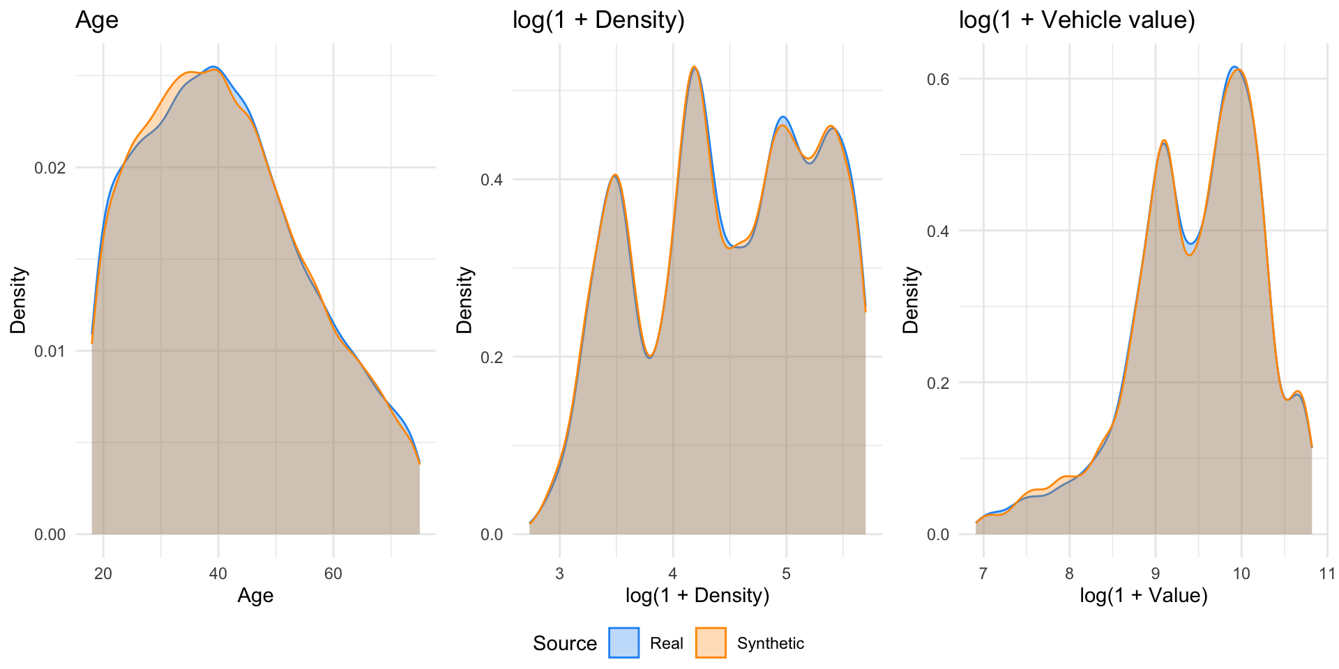
## Evaluating fidelity: marginal distributions
Do the synthetic marginals match the real data? `Age` is plotted on its raw scale, but `Density` (population density of the area where the car is kept) and `Value` (vehicle value) are plotted on a **log(1 + x)** scale. Both variables are heavily right-skewed: most policyholders live in low-to-moderate density areas and drive moderately priced vehicles, but a long tail of dense-urban locations and luxury vehicles stretches far beyond the bulk of the data. A raw-scale density plot would compress almost every record into a thin spike near zero, leaving the informative middle and tail of the distribution nearly invisible, and any real-vs-synthetic gap that mattered would be hidden inside that spike. The **`log1p()`** transform, $\log(1 + x)$ rather than plain $\log(x)$, compresses that long tail while remaining defined at $x = 0$ (plain $\log(0)$ is $-\infty$), which matters here since some records have `Density` or `Value` at or near zero.
```{r fidelity-marginals}
#| fig-cap: "Marginal distributions: real vs synthetic data."
#| fig-width: 10
#| fig-height: 5
compare_dfs <- bind_rows(
  df_synth_input %>% mutate(Source = "Real"),
  syn_df %>% mutate(Source = "Synthetic")
)

# Age is roughly symmetric, so the raw scale already shows the distribution clearly
p_age <- ggplot(compare_dfs, aes(x = Age, fill = Source, colour = Source)) +
  geom_density(alpha = 0.3) +
  scale_fill_manual(values = c("Real" = "#2196F3", "Synthetic" = "#FF9800")) +
  scale_colour_manual(values = c("Real" = "#2196F3", "Synthetic" = "#FF9800")) +
  labs(title = "Age", x = "Age", y = "Density") +
  theme_minimal() + theme(legend.position = "bottom")

# Density is right-skewed (a long tail of dense-urban locations), so log1p()
# spreads out the bulk of the data instead of compressing it into a spike near zero
p_density <- ggplot(compare_dfs, aes(x = log1p(Density), fill = Source, colour = Source)) +
  geom_density(alpha = 0.3) +
  scale_fill_manual(values = c("Real" = "#2196F3", "Synthetic" = "#FF9800")) +
  scale_colour_manual(values = c("Real" = "#2196F3", "Synthetic" = "#FF9800")) +
  labs(title = "log(1 + Density)", x = "log(1 + Density)", y = "Density") +
  theme_minimal() + theme(legend.position = "bottom")

# Vehicle value is right-skewed the same way (a long tail of luxury vehicles)
p_value <- ggplot(compare_dfs, aes(x = log1p(Value), fill = Source, colour = Source)) +
  geom_density(alpha = 0.3) +
  scale_fill_manual(values = c("Real" = "#2196F3", "Synthetic" = "#FF9800")) +
  scale_colour_manual(values = c("Real" = "#2196F3", "Synthetic" = "#FF9800")) +
  labs(title = "log(1 + Vehicle value)", x = "log(1 + Value)", y = "Density") +
  theme_minimal() + theme(legend.position = "bottom")

ggarrange(p_age, p_density, p_value, ncol = 3, common.legend = TRUE, legend = "bottom")
```
## Evaluating fidelity: summary statistics
```{r fidelity-stats}
#| results: asis
# Compare a handful of summary statistics side by side, real vs synthetic;
# close agreement here is a second, more targeted fidelity check than the
# full marginal-distribution plots above
fidelity_table <- tibble(
  Statistic = c(
    "Mean age", "SD age",
    "Claim frequency (% policies with claim)",
    "Mean claim amount (given claim)",
    "% Female",
    "Median vehicle value",
    "Mean density"
  ),
  Real = c(
    round(mean(df_synth_input$Age), 2),
    round(sd(df_synth_input$Age), 2),
    percent(mean(df_synth_input$Numtppd > 0), accuracy = 0.1),
    round(mean(df_synth_input$Indtppd[df_synth_input$Indtppd > 0]), 0),
    percent(mean(df_synth_input$Gender == "Female"), accuracy = 0.1),
    round(median(df_synth_input$Value), 0),
    round(mean(df_synth_input$Density), 0)
  ),
  Synthetic = c(
    round(mean(syn_df$Age), 2),
    round(sd(syn_df$Age), 2),
    percent(mean(syn_df$Numtppd > 0), accuracy = 0.1),
    round(mean(syn_df$Indtppd[syn_df$Indtppd > 0]), 0),
    percent(mean(syn_df$Gender == "Female"), accuracy = 0.1),
    round(median(syn_df$Value), 0),
    round(mean(syn_df$Density), 0)
  )
)

fidelity_table %>%
  kable(caption = "Fidelity check: real vs synthetic data statistics") %>%
  kable_styling(font_size = 12)
```
## Evaluating fidelity: model coefficients
A further fidelity test is whether a model trained on synthetic data recovers similar fitted relationships to one trained on real data. This compares model coefficients directly, rather than predictive performance on held-out data, which the next section tests directly.
```{r fidelity-model}
#| code-fold: true
#| code-summary: "Train and compare GLMs on real vs synthetic data"
#| results: asis
library(MASS)  # for glm.nb if needed

# Same claim-frequency GLM specification fit twice, once on each dataset;
# Density and Value are log1p()-transformed for the same right-skew reason
# discussed above, this time as GLM predictors rather than plot axes
fit_claim_model <- function(df) {
  glm(
    (Numtppd > 0) ~ Age + Gender + log1p(Density) + log1p(Value) + Bonus,
    family  = binomial(link = "logit"),
    data    = df
  )
}

model_real <- fit_claim_model(df_synth_input)
model_syn  <- fit_claim_model(syn_df)

# If synthesis preserved the real relationships well, these coefficients
# should be close, not just the marginal distributions from earlier
coef_comparison <- tibble(
  Coefficient = names(coef(model_real)),
  `Real data`      = round(coef(model_real), 4),
  `Synthetic data` = round(coef(model_syn), 4),
  `Difference`     = round(coef(model_syn) - coef(model_real), 4)
) %>%
  filter(Coefficient != "(Intercept)")

coef_comparison %>%
  kable(caption = "Logistic regression coefficients: real vs synthetic data") %>%
  kable_styling(font_size = 11)
```
## Evaluating utility: train-synthetic-test-real (TSTR)
Coefficient agreement checks whether the synthetic data *resembles* the real data. It does not answer the question a data user actually cares about: if this synthetic data were used to build a production model, how well would that model perform on real, future records? The standard way to test this is **train-synthetic-test-real (TSTR)**: fit a model on synthetic data, then evaluate it on real records the synthesis process never saw, here, the 2,000-record `df_real_holdout` set aside earlier. We compare this against the natural benchmark: the same model fitted on real training data, evaluated on that same real holdout.
```{r tstr}
#| results: asis
# Area under the ROC curve (AUC), computed from ranks rather than a package:
# AUC = P(a random positive scores higher than a random negative), which the
# sum of ranks among the positive cases estimates directly (Mann-Whitney U).
auc_manual <- function(pred, actual) {
  n1 <- sum(actual == 1)
  n0 <- sum(actual == 0)
  r  <- rank(pred)
  (sum(r[actual == 1]) - n1 * (n1 + 1) / 2) / (n1 * n0)
}

holdout_actual <- as.integer(df_real_holdout$Numtppd > 0)

# Same two models fitted above (model_real on real data, model_syn on
# synthetic data), now scored on real records neither model was trained on
pred_from_real_model <- predict(model_real, newdata = df_real_holdout, type = "response")
pred_from_syn_model  <- predict(model_syn,  newdata = df_real_holdout, type = "response")

tibble(
  `Model trained on` = c("Real data", "Synthetic data"),
  `AUC on real holdout` = c(
    round(auc_manual(pred_from_real_model, holdout_actual), 4),
    round(auc_manual(pred_from_syn_model,  holdout_actual), 4)
  )
) %>%
  kable(caption = "Train-synthetic-test-real (TSTR): predictive performance on 2,000 held-out real records") %>%
  kable_styling(font_size = 12)
```
**Reading this table.** Both rows are scored on the exact same real, held-out records, so this is a fair comparison of what each training data source actually delivers downstream. Here the two AUCs are 0.728 (real) and 0.729 (synthetic), a negligible, and if anything reversed, gap: a model built entirely on synthetic data performs just as well, on real future business, as one built on the real data it was meant to protect. That is stronger evidence than coefficient agreement alone, since it directly tests the thing a downstream user would do with the data, rather than a large gap, which would mean the coefficient-level agreement above was optimistic: close average coefficients do not guarantee close predictive performance once a model has to generalise to records it has never seen.
## Evaluating privacy: nearest-neighbour distance
A synthetic dataset that copies real records verbatim offers no privacy protection. The **nearest-neighbour distance ratio** (NNDR) measures how close synthetic records are to real ones:
$$\text{NNDR} = \frac{d(\text{syn}_i, \text{real nearest})}{d(\text{syn}_i, \text{real 2nd nearest})}$$
A NNDR close to 1 means the nearest real record is no closer than the second-nearest, so the synthetic record is not a copy. A NNDR close to 0 suggests memorisation.
**Why the ratio, not just the raw distance to the nearest real record.** Checking raw distance alone would be misleading, because it does not account for local density. In a crowded region of the data (common combinations of `Age`, `Density`, `Value`), *every* nearby point, including a synthetic record that copied nothing, will naturally sit close to some real record, simply because real records are packed tightly there. That is not leakage, it is geometry. Dividing by the distance to the *second*-nearest real record normalises for this: in a dense region, the nearest and second-nearest real records are both close and roughly similar in distance to each other, so the ratio stays near 1, the synthetic point is not suspiciously attached to any one record, it is just sitting in a crowded part of the distribution, as it should. If a synthetic record is instead a near-copy of one specific real record, its nearest-neighbour distance collapses toward zero while its second-nearest distance stays at the normal local scale, and the ratio collapses toward 0. That is the density-normalised signal that something specific, not just "nearby data exists", is happening.
NNDR is, even so, a narrow test: it only checks exact-or-near-exact geometric proximity on the specific numeric columns included in the distance calculation (`Age`, `Density`, `Value` below, not the categorical columns). It says nothing about **membership inference** (could an attacker determine a specific real person was in the training data without any single synthetic record being suspiciously close, for instance from aggregate statistical signatures) or **attribute inference** (could an attacker infer a sensitive attribute about someone from the synthetic data as a whole, without any record-level match at all). It is a cheap, useful first-pass diagnostic for one specific failure mode, memorisation, not a privacy guarantee in the way differential privacy's mathematical bound is.
```{r privacy-nndr}
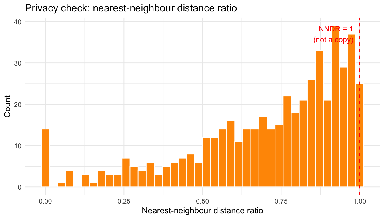
#| fig-cap: "Distribution of nearest-neighbour distance ratios. Values near 1 indicate the synthetic data is not copying real records."
#| fig-width: 7
#| fig-height: 4
# Standardise numeric columns for distance computation
num_cols <- c("Age", "Density", "Value")

real_scaled <- scale(df_synth_input[, num_cols])
syn_scaled  <- scale(syn_df[, num_cols],
                     center = attr(real_scaled, "scaled:center"),
                     scale  = attr(real_scaled, "scaled:scale"))

# Sample 500 synthetic records for speed
idx <- sample(nrow(syn_scaled), 500)
syn_sample <- syn_scaled[idx, ]

# Compute distances to real data
dist_mat <- as.matrix(dist(rbind(syn_sample, real_scaled)))[
  seq_len(nrow(syn_sample)),
  (nrow(syn_sample) + 1):(nrow(syn_sample) + nrow(real_scaled))
]

nn1 <- apply(dist_mat, 1, function(d) sort(d)[1])
nn2 <- apply(dist_mat, 1, function(d) sort(d)[2])
nndr <- nn1 / nn2

ggplot(tibble(nndr = nndr), aes(x = nndr)) +
  geom_histogram(bins = 40, fill = "#FF9800", colour = "white") +
  geom_vline(xintercept = 1, linetype = "dashed", colour = "red") +
  annotate("text", x = 0.98, y = Inf, label = "NNDR = 1\n(not a copy)",
           vjust = 1.5, hjust = 1, colour = "red", size = 3.5) +
  labs(x = "Nearest-neighbour distance ratio",
       y = "Count",
       title = "Privacy check: nearest-neighbour distance ratio") +
  theme_minimal()
```
## Reading the NNDR plot
- Most synthetic records have NNDR near 1. The nearest and second-nearest real records are approximately equidistant. **The synthetic data is not copying real records.**
- There is a genuine spike near NNDR = 0: about 4% of the sampled synthetic records (20 of 500) have a real record at distance exactly zero on `Age`, `Density`, and `Value`. This is not full-record memorisation. `synthpop`'s CART method draws each numeric value from the *actual observed values* in the matching leaf of its fitted tree rather than smoothing or adding noise, so a synthetic record's `Age`/`Density`/`Value` combination can coincidentally match one specific real record's combination exactly, particularly since `Density` in this dataset takes only 471 distinct values across 8,000 records. Checking these exact-match cases shows the categorical variables (`Group1`, `Bonus`) and the claim outcome still typically differ between the synthetic record and its numeric near-match, so the record as a whole is not a copy, but an exact match on continuous-looking variables that turn out to have limited real-world cardinality is exactly the kind of residual risk the membership-inference testing mentioned below is designed to catch.
- `synthpop` with CART generally achieves good NNDR because CART introduces randomness at each leaf when `minbucket` > 1.
::: {.callout-important}
NNDR on numeric columns is only one test. A complete privacy evaluation also checks **membership inference** (can an attacker determine whether a given record was in the training data?) and **attribute inference** (can an attacker infer a sensitive variable?). See @jordon2022synthetic for a full evaluation framework.
:::
# Lifecycle controls
## Putting it together: controls by stage
```{r controls-table}
#| results: asis
# Reference table, not derived from the analysis above: maps each stage of
# the data lifecycle to the controls and regulatory hooks (APP/GDPR) that apply
tibble(
  `Stage` = c("Collection", "Storage", "Analytics / modelling",
               "Output / sharing", "Retention / deletion"),
  `Key controls` = c(
    "Collect minimum necessary; document legal basis; notify individuals (APP 3, 5; GDPR Art 5–6)",
    "Pseudonymise identifiers; encrypt at rest; role-based access; audit logs (APP 11; GDPR Art 25)",
    "Purpose limitation; k-anonymise or apply DP before analyst access; synthetic data for dev/test (APP 6; GDPR Art 5)",
    "Aggregate statistics only; DP noise on releases; data sharing agreements; vendor due diligence (APP 8; GDPR Art 28)",
    "Automated deletion at end of retention period; secure disposal; document destruction (APP 11; GDPR Art 5)"
  )
) %>%
  kable(caption = "Privacy controls by data lifecycle stage") %>%
  kable_styling(font_size = 11) %>%
  column_spec(1, bold = TRUE, width = "8em") %>%
  column_spec(2, width = "30em")
```
## Choosing the right technique
```{r technique-choice}
#| results: asis
# Reference table summarising when to reach for each PET covered in this lecture
tibble(
  Technique = c("Pseudonymisation", "k-Anonymity", "Differential privacy", "Synthetic data"),
  `Best for` = c(
    "Separating identifiers from analytics data within the organisation",
    "Publishing tabular statistics or micro-data with few quasi-identifiers",
    "Releasing aggregate statistics or training models on sensitive datasets",
    "Sharing realistic datasets externally; testing pipelines; rare-event augmentation"
  ),
  `Main limitation` = c(
    "Does not protect against re-identification if the key file is compromised",
    "Breaks down with many quasi-identifiers or continuous variables",
    "Requires careful calibration of ε; reduces utility; composition across queries",
    "Fidelity may be poor for rare subgroups; requires privacy evaluation"
  )
) %>%
  kable(caption = "Privacy technique selection guide") %>%
  kable_styling(font_size = 11) %>%
  column_spec(1, bold = TRUE, width = "8em")
```
::: {.callout-note title="Case study, resolved: answering the three opening questions"}
**Question 1: Which recipient could you defensibly hand k-anonymised data to? Does the reinsurer's partial background knowledge change your answer?**
Arguably none of the three, though not because k-anonymity is broken, it is simply the wrong tool for all three specific requests here. The reinsurer needs realistic, record-level data to build an independent model, which k-anonymity degrades rather than provides; the internal team does not need a degraded file at all; the vendor does not need a file at all. Where k-anonymity would otherwise apply, background knowledge does change the answer: this chapter's own $k=50$ result left `Gender`, `AgeGroup`, and `DensityGroup`, exactly the variables a reinsurer with prior treaty-year exposure might already know, completely untouched by suppression, so the "hides among $k$ others" argument is weaker for precisely this recipient than for a blind outsider.
**Question 2: Does the pricing team's need for realistic (not real) data argue for synthetic data, or is there a simpler answer?**
The simpler answer: no PET at all, just governance. The pricing team is internal, already bound by confidentiality obligations, and its model will be validated against live production data regardless of what it is trained on. Spending synthesis effort to serve a recipient who does not need it, and who gains nothing privacy-wise from data that is already inside the organisation, is effort misapplied. Purpose limitation and role-based access, the "Analytics / modelling" row of the lifecycle-controls table below, is the proportionate control.
**Question 3: Does the vendor's aggregate-only need rule out two of the chapter's three techniques?**
Yes. k-anonymity and synthetic data both exist to protect a *file* of records; the vendor never receives one. That leaves **differential privacy** as the only relevant technique of the three, and this chapter's own results showed that, at this portfolio's scale, strong privacy (small $\varepsilon$) costs the vendor essentially nothing in accuracy for a portfolio-wide statistic, provided the regulator does not later ask for a finer breakdown of a small subgroup.
**In short:** synthetic data for the reinsurer (TSTR: AUC 0.728 vs. 0.729, subject to the membership-inference caveat raised earlier), governance alone for the internal team, differential privacy for the vendor. Three recipients, three different tools, not one technique applied uniformly.
:::
# Summary
- **Re-identification risk** is real even in large, "anonymised" datasets. Quasi-identifier combinations can uniquely identify rare groups, and the same risk-assessment workflow (identify quasi-identifiers → choose a matched PET → apply → measure trade-off → decide) transfers to other domains.
- **k-Anonymity** via local suppression reduces identifiability but does not protect sensitive values, and the utility cost rises sharply once $k$ is large enough to force real suppression, not just at the textbook-minimum $k = 5$.
- **Differential privacy** provides a mathematical guarantee and scales well to large datasets: the same $\varepsilon$ that leaves a 100,000-record aggregate nearly untouched can distort a small subgroup significantly, because sensitivity scales as $1/n$. The Laplace mechanism is straightforward to implement for aggregate statistics.
- **Synthetic data** from `synthpop` (CART) achieves good fidelity on marginals and model coefficients, a model trained on it generalises to held-out real records nearly as well as one trained on real data (TSTR), and NNDR evidence shows real records are not being copied.
- No single technique is sufficient on its own — **layered controls** across the data lifecycle are required.
# Recommended reading
**Re-identification risk and k-anonymity**
- @templ2017statistical — `sdcMicro` and statistical disclosure control
- @sweeney2002kanonymity — k-anonymity
- @machanavajjhala2007diversity — ℓ-diversity (extension of k-anonymity)
**Differential privacy and synthetic data**
- @dwork2006calibrating — original ε-differential privacy paper
- @nowok2016synthpop — `synthpop` R package and CART synthesis
- @jordon2022synthetic — synthetic data: what, why and how (evaluation framework)